Case Study: Zhongshan Land Subsidence Uncertainty

Context: Forecasting in Complex Urban Environments

Urban areas, particularly coastal and delta regions like Zhongshan in China’s Pearl River Delta, face significant challenges from land subsidence. This gradual sinking, driven by complex interactions between groundwater extraction, geological conditions, infrastructure load, and climate factors, poses risks to buildings, flood control, and sustainable development. Accurately forecasting future subsidence is crucial for effective urban planning and hazard mitigation, but requires not only predicting the most likely outcome but also understanding the associated predictive uncertainty (Liu et al.[1]).

This case study demonstrates how various visualization tools within the k-diagram package can be applied to analyze and interpret the outputs of a land subsidence forecasting model, using a sample dataset derived from research focused on the Zhongshan area (Kouadio[2]). We will explore how different polar plots help reveal patterns in uncertainty, model performance, and potential prediction anomalies.

Note

The dataset used in this case study (min_zhongshan.csv, accessed via load_zhongshan_subsidence()) is a sample derived from larger research model outputs. It is provided for educational and demonstration purposes only to illustrate the use of k-diagram functions. It does not represent the complete, validated forecast results for the region.

The Zhongshan Sample Dataset

The dataset included with k-diagram provides a snapshot of predicted subsidence uncertainty for 898 locations over multiple years.

Key Characteristics:

• Spatial Coordinates: Includes longitude and latitude for each location.

• Target Values: Contains columns subsidence_2022 and subsidence_2023 representing reference or baseline subsidence values for those years (useful for some diagnostics like coverage).

• Quantile Forecasts: Provides predicted quantiles (Q10, Q50, Q90) for the years 2022 through 2026 (e.g., subsidence_2024_q0.1, subsidence_2024_q0.5, subsidence_2024_q0.9). This allows analysis of uncertainty intervals and their evolution over time.

Loading the Data:

You can easily load this data using the provided function. By default, it returns a Bunch object containing the DataFrame and useful metadata:

import kdiagram as kd
import warnings

# Ignore potential download/cache warnings for brevity
warnings.filterwarnings("ignore", message=".*already exists.*")

# Load data as Bunch (default)
try:
    zhongshan_data = kd.datasets.load_zhongshan_subsidence(
        download_if_missing=True # Allow download if not found
    )
    print("Zhongshan data loaded successfully.")
    print(f"DataFrame shape: {zhongshan_data.frame.shape}")
    print("\nAvailable Columns (Sample):")
    print(zhongshan_data.frame.columns[:10].tolist(), "...") # Show some columns
    # print(zhongshan_data.DESCR) # Uncomment to see full description
except FileNotFoundError:
    print("Zhongshan dataset not found. Ensure k-diagram is installed"
          " correctly with data, or check internet connection.")

Example Output

Loading dataset from cache: ... or Loading dataset from installed package...
Zhongshan data loaded successfully.
DataFrame shape: (898, 19)

Available Columns (Sample):
['longitude', 'latitude', 'subsidence_2022', 'subsidence_2023', 'subsidence_2022_q0.1', 'subsidence_2022_q0.5', 'subsidence_2022_q0.9', 'subsidence_2023_q0.1', 'subsidence_2023_q0.5', 'subsidence_2023_q0.9'] ...

Analysis Examples using k-diagram

The following sections demonstrate how different k-diagram plots can be used with the Zhongshan dataset sample to analyze various aspects of the forecast uncertainty and model behavior.

---

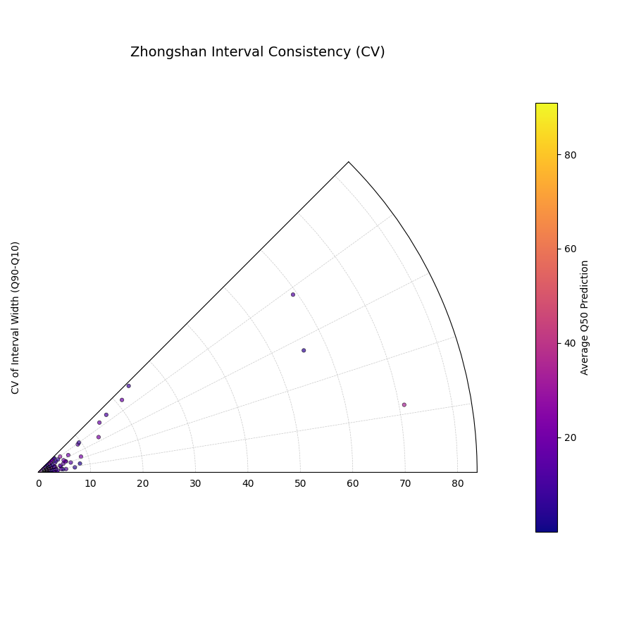
Loading Zhongshan Data for Interval Consistency Plot

This example demonstrates loading the packaged Zhongshan dataset using load_zhongshan_subsidence() (as a Bunch object) and analyzing the temporal consistency of its prediction interval widths using plot_interval_consistency(). Includes basic error handling in case the data cannot be loaded.

import kdiagram as kd
import matplotlib.pyplot as plt
import warnings
import pandas as pd # Used by the function internally

# Suppress potential download warnings if data exists locally
warnings.filterwarnings("ignore", message=".*already exists.*")

ax = None # Initialize ax
try:
    # 1. Load data as Bunch, allow download if missing
    data = kd.datasets.load_zhongshan_subsidence(
        as_frame=False,
        download_if_missing=True,
    )

    # 2. Check if data loaded and has necessary columns
    if (data is not None and hasattr(data, 'frame')
            and data.q10_cols and data.q50_cols and data.q90_cols):

        print(f"Loaded Zhongshan data with {len(data.frame)} samples.")
        print(f"Plotting consistency for {len(data.q10_cols)} periods.")

        # 3. Create the Interval Consistency plot
        ax = kd.plot_interval_consistency(
            df=data.frame,
            qlow_cols=data.q10_cols,
            qup_cols=data.q90_cols,
            q50_cols=data.q50_cols, # Use Q50 for color context
            use_cv=True,           # Use Coefficient of Variation
            title="Zhongshan Interval Consistency (CV)",
            cmap='plasma',
            s=15, alpha=0.7,
            acov='eighth_circle',
            mask_angle=True,
            # Save the plot
            savefig="../images/dataset_plot_example_zhongshan_consistency.png"
        )
        plt.close() # Close plot after saving
    else:
        print("Loaded data object missing required attributes (frame/cols).")

except FileNotFoundError as e:
    print(f"ERROR - Zhongshan data not found: {e}")
except Exception as e:
    print(f"An unexpected error occurred during plotting: {e}")

if ax is None:
    print("Plot generation skipped due to data loading issues.")

🧠 Analysis and Interpretation

This plot uses plot_interval_consistency() to assess the stability of the predicted uncertainty range (Q90-Q10 interval width) over time (2022-2026) for the Zhongshan sample dataset. The plot is restricted to a 45-degree angular sector (acov='eighth_circle').

Analysis and Interpretation:

• Angle (θ): Represents a subset of the location indices (0-897) mapped onto a 45-degree arc. Labels are masked.

• Radius (r): Shows the Coefficient of Variation (CV) of the interval width (Q90-Q10) calculated across the years 2022-2026 for each location. A higher radius indicates greater relative variability in the predicted uncertainty width over time for that location.

• Color: Represents the average Q50 (median subsidence prediction) across all years for each location, using the plasma colormap (purple=low, yellow=high). The color bar indicates the scale.

🔍 Key Insights from this Example:

• High General Consistency: The vast majority of points are clustered very close to the center (radius near 0), indicating a very low CV. This suggests that for most locations in this sample and view, the width of the predicted uncertainty interval is relatively stable and consistent across the forecast horizon (2022-2026).

• Outliers: A few distinct points have a significantly larger radius (CV > 40). These represent locations where the predicted interval width fluctuates dramatically over the years relative to its average width, signaling highly inconsistent or unstable uncertainty predictions.

• Color Context: The dense cluster of consistent points (low CV) mainly shows purple and dark blue colors, corresponding to lower average Q50 predictions. The few highly inconsistent points (high CV outliers) show a mix of colors, suggesting instability can occur at different average subsidence levels in this dataset.

💡 Use Case Connection:

• This plot helps identify specific locations (the outliers) where the model’s uncertainty predictions are unreliable over time, warranting further investigation.

• The general consistency for most points (low CV cluster) might increase confidence in the stability of uncertainty estimates for those areas, potentially aiding risk assessment where the average predicted subsidence (color) is also low.

---

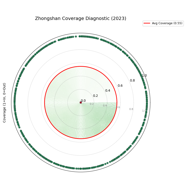
Loading Zhongshan Data for Coverage Diagnostic (Specific Year)

This example loads the Zhongshan dataset, subsets it to a specific year (2023) and relevant quantiles (Q10, Q90) during the load step, and then uses plot_coverage_diagnostic() to visualize point-wise coverage for that year.

import kdiagram as kd
import matplotlib.pyplot as plt
import warnings
import pandas as pd

# Suppress potential download warnings
warnings.filterwarnings("ignore", message=".*already exists.*")

ax = None
try:
    # 1. Load data as Bunch, selecting only 2023 data and Q10/Q90
    # Also ensure the target column for 2023 is included.
    # Note: Target column name is 'subsidence_2023' in this dataset.
    data = kd.datasets.load_zhongshan_subsidence(
        as_frame=False,
        years=[2023],            # Select only year 2023
        quantiles=[0.1, 0.9],    # Select only Q10 and Q90
        include_target=True,     # Ensure target column is kept
        download_if_missing=True
    )

    # 2. Check data and identify columns for plotting
    actual_col = 'subsidence_2023' # Known target column for 2023
    q_cols_plot = []
    if data is not None and actual_col in data.frame.columns:
         if data.q10_cols: q_cols_plot.append(data.q10_cols[0])
         if data.q90_cols: q_cols_plot.append(data.q90_cols[0])

    if len(q_cols_plot) == 2:
        print(f"Loaded Zhongshan data for {actual_col}.")
        print(f"Plotting coverage diagnostic using: {q_cols_plot}")

        # 3. Create the Coverage Diagnostic plot
        ax = kd.plot_coverage_diagnostic(
            df=data.frame,
            actual_col=actual_col,
            q_cols=q_cols_plot, # Should contain 2023 Q10 & Q90 cols
            title="Zhongshan Coverage Diagnostic (2023)",
            as_bars=False, # Use scatter points
            fill_gradient=True,
            verbose=1, # Print overall coverage rate
            # Save the plot
            savefig="../images/dataset_plot_example_zhongshan_coverage.png"
        )
        plt.close()
    else:
         print("Required columns ('subsidence_2023', Q10, Q90) "
               "not found in loaded data.")

except FileNotFoundError as e:
    print(f"ERROR - Zhongshan data not found: {e}")
except Exception as e:
    print(f"An unexpected error occurred: {e}")

if ax is None:
    print("Plot generation skipped.")

🧠 Analysis and Interpretation

This plot uses plot_coverage_diagnostic() to assess the point-wise coverage of the Q10-Q90 prediction interval against the target subsidence_2023 values from the Zhongshan sample dataset for the year 2023.

Analysis and Interpretation:

• Angle (θ): Represents the index (0-897) of each specific location in the Zhongshan dataset, mapped around the circle.

• Radius (r): Indicates coverage: 1 if the actual 2023 subsidence value was within the predicted [Q10, Q90] interval for that location; 0 if it was outside.

• Points: Scatter points (as_bars=False) are used. The vast majority appear clustered at radius 1 (greenish points). Points at radius 0 (uncovered) are difficult to discern visually in this rendering, possibly due to overlap or marker style.

• Average Coverage Line: The solid red line forms a circle at a radius corresponding to the overall coverage rate, explicitly labeled in the legend as 0.55 (or 55%).

• Gradient Fill: The green shaded area extends from the center only up to the average coverage radius (0.55).

🔍 Key Insights from this Example:

• Significant Under-coverage: The most striking feature is the low average coverage rate of 55% (indicated by the red line and legend), despite using a nominal 80% prediction interval (Q10-Q90). This suggests the model’s prediction intervals for 2023 were, on average, too narrow and failed to capture the true subsidence value almost half the time for this dataset.

• Visual vs. Average Discrepancy: While visually most plotted points seem to indicate success (radius 1), the calculated average (55%) reveals that a substantial number of points must be at radius 0 (uncovered), even if not clearly visible. This highlights the importance of the calculated average line as a reliable summary statistic.

• Potential Issues: The low coverage rate indicates potential issues with the model’s uncertainty calibration for the 2023 forecast period in the original study this sample data is derived from.

💡 When to Use:

• Use this plot to verify if the prediction intervals for a specific time period achieve the desired nominal coverage.

• Identify if coverage failures are widespread (as suggested by the low average here) or specific to certain samples (which would require examining the points near radius 0 more closely, perhaps with different marker styles or alpha settings).

• Assess the practical reliability of the forecast’s uncertainty bounds for decision-making in a given period.

---

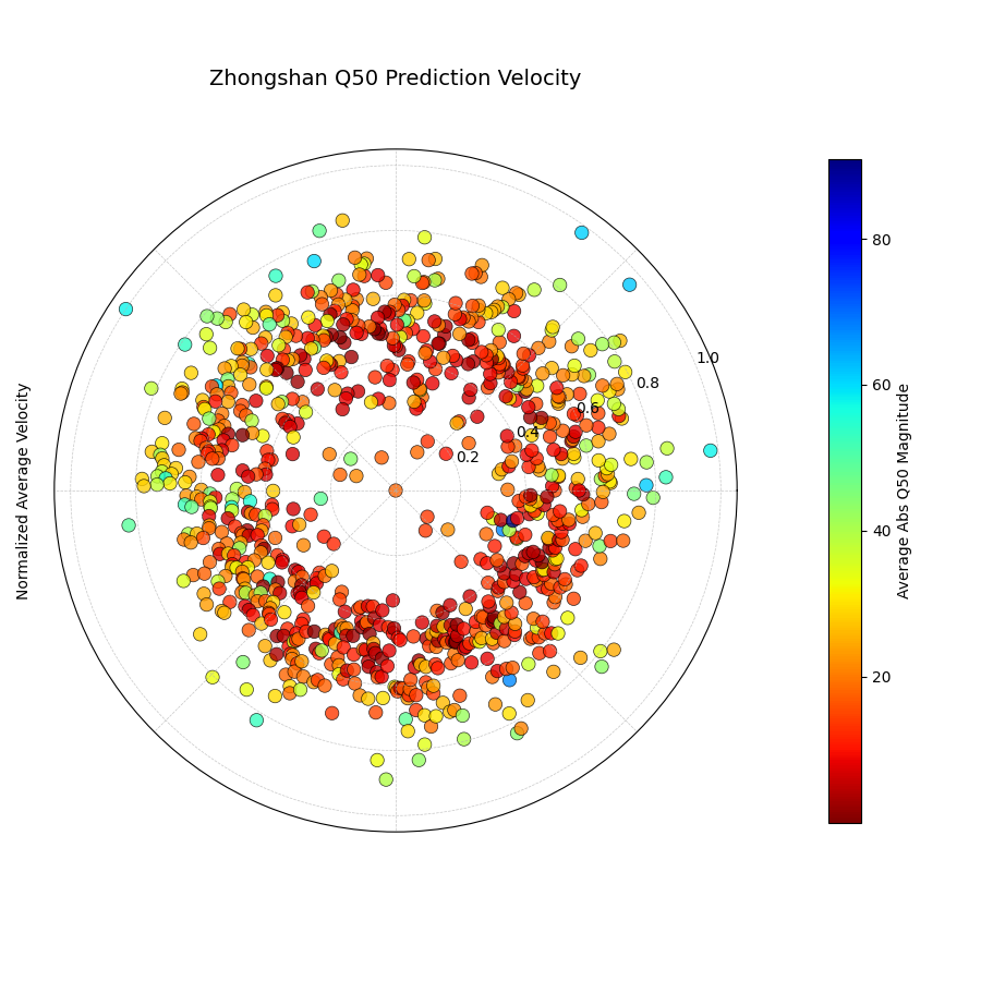
Zhongshan Data: Velocity Plot (Default Coverage)

Load Zhongshan data (as Bunch) and visualize the average velocity of the median (Q50) predictions using the full 360-degree view (acov=’default’). Color represents the average Q50 magnitude.

import kdiagram as kd
import matplotlib.pyplot as plt
import warnings
import pandas as pd

warnings.filterwarnings("ignore", message=".*already exists.*")
ax = None
try:
    # 1. Load data as Bunch
    data = kd.datasets.load_zhongshan_subsidence(
        as_frame=False, download_if_missing=True
        )

    # 2. Check data
    if data is not None and data.q50_cols:
        print(f"Loaded Zhongshan data with {len(data.frame)} samples.")
        print(f"Plotting velocity using {len(data.q50_cols)} periods.")

        # 3. Create the Velocity plot
        ax = kd.plot_velocity(
            df=data.frame,
            q50_cols=data.q50_cols,
            title="Zhongshan Q50 Prediction Velocity",
            acov='default',       # Full circle coverage
            use_abs_color=True,   # Color by Q50 magnitude
            normalize=True,       # Normalize radius
            cmap='jet_r',
            cbar=True, s=80, alpha=0.8,
            mask_angle=True,
            # Save the plot
            savefig="../images/dataset_plot_example_zhongshan_velocity.png"
        )
        plt.close()
    else:
        print("Loaded data object missing required attributes.")

except FileNotFoundError as e:
    print(f"ERROR - Zhongshan data not found: {e}")
except Exception as e:
    print(f"An unexpected error occurred: {e}")

if ax is None: print("Plot generation skipped.")

🧠 Analysis and Interpretation

This plot, generated by plot_velocity(), visualizes the average rate of change (velocity) of the median (Q50) subsidence predictions across the available years (likely 2022-2026) for each location in the Zhongshan sample dataset.

Analysis and Interpretation:

• Angle (θ): Represents the index (0-897) of each location, distributed around the full 360 degrees (acov='default'). Angular labels are hidden (mask_angle=True).

• Radius (r): Shows the normalized average velocity, scaled to [0, 1] (due to normalize=True). A radius near 1 indicates locations where the Q50 prediction changed most rapidly on average over the years; a radius near 0 indicates very stable Q50 predictions.

• Color: Represents the average absolute Q50 magnitude across all years for each location (since use_abs_color=True). The jet_r colormap is used (blue=low magnitude, red=high magnitude), with the scale shown on the color bar.

• Marker Size/Alpha: Larger markers (s=80) with some transparency (alpha=0.8) are used.

🔍 Key Insights from this Example:

• Velocity Distribution: There is a considerable spread in velocities. While many locations show low to moderate normalized velocity (points clustered r < 0.5), a noticeable number exhibit higher velocities (points with r > 0.6), indicating significant variation in the predicted rate of subsidence change across locations.

• Velocity vs. Magnitude: Visually, there appears to be some correlation between velocity and magnitude. Locations with higher average Q50 magnitude (yellow/orange/red points) seem more prevalent at larger radii (higher velocity) compared to locations with lower average Q50 (blue/cyan points), which are more concentrated near the center (lower velocity). This suggests areas predicted to have higher subsidence might also be predicted to change more rapidly.

• Spatial Pattern: Without angular labels tied to actual spatial coordinates, identifying precise geographical patterns is hard, but the overall distribution appears somewhat uniform angularly, without extreme clustering in specific index ranges.

💡 Use Case Connection:

• This plot helps identify locations within the Zhongshan sample predicted to undergo the fastest average rate of change in subsidence over the forecast period (points furthest from center).

• By coloring by average Q50 magnitude, it allows planners to see if these high-velocity areas are also areas of high absolute subsidence risk, potentially requiring priority attention.

---

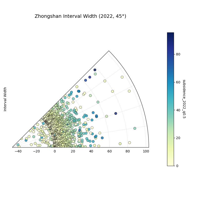
Zhongshan Data: Interval Width Plot (2022, Eighth Circle)

Load Zhongshan data, select the Q10, Q50, and Q90 columns for the first available year (assumed 2022), and plot the interval width using plot_interval_width() with Q50 for color, restricted to a 45-degree view (acov=’eighth_circle’).

import kdiagram as kd
import matplotlib.pyplot as plt
import warnings
import pandas as pd

warnings.filterwarnings("ignore", message=".*already exists.*")
ax = None
try:
    # 1. Load data as Bunch
    data = kd.datasets.load_zhongshan_subsidence(
        as_frame=False, download_if_missing=True
        )

    # 2. Check data and extract columns for the first year (e.g., 2022)
    if (data is not None and hasattr(data, 'frame')
            and data.q10_cols and data.q50_cols and data.q90_cols):

        q10_col_first = data.q10_cols[0] # Assumes list is ordered
        q50_col_first = data.q50_cols[0]
        q90_col_first = data.q90_cols[0]
        year_first = str(data.start_year) # Assumes start_year attr exists

        print(f"Plotting interval width for Zhongshan, year {year_first}")

        # 3. Create the Interval Width plot
        ax = kd.plot_interval_width(
            df=data.frame,
            q_cols=[q10_col_first, q90_col_first], # Q10, Q90 for one year
            z_col=q50_col_first,       # Color by Q50 of that year
            acov='eighth_circle',      # <<< Use 45 degree view
            title=f"Zhongshan Interval Width ({year_first}, 45°)",
            cmap='YlGnBu',
            cbar=True, s=55, alpha=0.85, mask_angle=True,
            # Save the plot
            savefig="../images/dataset_plot_example_zhongshan_width_45deg.png"
        )
        plt.close()
    else:
        print("Loaded data object missing required attributes.")

except FileNotFoundError as e:
    print(f"ERROR - Zhongshan data not found: {e}")
except Exception as e:
    print(f"An unexpected error occurred: {e}")

if ax is None: print("Plot generation skipped.")

🧠 Analysis and Interpretation

This plot uses plot_interval_width() to display the magnitude of the predicted uncertainty (interval width) for the year 2022 in the Zhongshan sample dataset. The view is restricted to a 45-degree sector (acov='eighth_circle').

Analysis and Interpretation:

• Angle (θ): Represents a subset of the location indices mapped onto the 45-degree arc. Angular labels are hidden.

• Radius (r): Directly shows the raw interval width calculated as subsidence_2022_q90 - subsidence_2022_q10 for each plotted location. Larger radius indicates greater predicted uncertainty magnitude for 2022.

• Color: Represents the median prediction value (subsidence_2022_q50) for each location, using the YlGnBu colormap (light yellow/green = low Q50, dark blue = high Q50), indicated by the color bar.

🔍 Key Insights from this Example:

• Width Distribution: For the locations visible in this narrow sector, most prediction intervals in 2022 have widths ranging roughly from 0 to 40 units.

• Width vs. Magnitude: Within the main cluster, there isn’t an immediately obvious strong correlation between interval width (radius) and the median prediction Q50 (color) – various widths appear across different Q50 levels.

• Outliers & Potential Data Issues: Several points exhibit very large positive radii (high uncertainty), and notably, some points have negative radii (plotted below the center). Negative radii imply that for those specific locations in the 2022 data sample, the recorded Q10 value was greater than the Q90 value, which indicates either a data error or a severe model prediction failure for those points.

💡 When to Use / Connection:

• Use this plot to directly visualize the predicted uncertainty magnitude (interval width) for each sample at a single point in time.

• The color mapping (z_col) helps investigate relationships between uncertainty width and the central tendency (Q50) or other features.

• Identifying outliers with extremely large or physically implausible (negative) widths is crucial for model diagnostics and data quality checks. These specific locations from the Zhongshan sample would require further investigation in a real analysis.

• Using narrower acov settings like eighth_circle can help focus on specific subsets if the angular arrangement is meaningful, but limits the overall view.

---

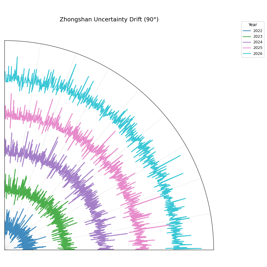
Zhongshan Data: Uncertainty Drift Plot (Quarter Circle)

Load Zhongshan data (as Bunch) and visualize the temporal drift of uncertainty patterns using concentric rings with plot_uncertainty_drift(), restricted to a 90-degree view (acov=’quarter_circle’).

import kdiagram as kd
import matplotlib.pyplot as plt
import warnings
import pandas as pd

warnings.filterwarnings("ignore", message=".*already exists.*")
ax = None
try:
    # 1. Load data as Bunch
    data = kd.datasets.load_zhongshan_subsidence(
        as_frame=False, download_if_missing=True
        )

    # 2. Check data and prepare labels
    if (data is not None and hasattr(data, 'frame')
            and data.q10_cols and data.q90_cols
            and hasattr(data, 'start_year') and hasattr(data, 'n_periods')):

        horizons = [str(data.start_year + i) for i in range(data.n_periods)]
        print(f"Plotting uncertainty drift for Zhongshan: {horizons}")

        # 3. Create the Uncertainty Drift plot
        ax = kd.plot_uncertainty_drift(
            df=data.frame,
            qlow_cols=data.q10_cols,
            qup_cols=data.q90_cols,
            dt_labels=horizons,
            acov='quarter_circle', # <<< Use 90 degree view
            title="Zhongshan Uncertainty Drift (90°)",
            cmap='viridis',
            show_legend=True, mask_angle=True,
            # Save the plot
            savefig="../images/dataset_plot_example_zhongshan_uncertainty_drift.png"
        )
        plt.close()
    else:
        print("Loaded data object missing required attributes.")

except FileNotFoundError as e:
    print(f"ERROR - Zhongshan data not found: {e}")
except Exception as e:
    print(f"An unexpected error occurred: {e}")

if ax is None: print("Plot generation skipped.")

🧠 Analysis and Interpretation

This plot uses plot_uncertainty_drift() to visualize how the pattern of predicted uncertainty (relative interval width Q90-Q10) evolves over multiple years (2022-2026) for the Zhongshan sample dataset. The view is focused on a 90-degree sector (acov='quarter_circle').

Analysis and Interpretation:

• Angle (θ): Represents a subset of the location indices (0-897) mapped onto the 90-degree arc. Angular labels are hidden (mask_angle=True).

• Concentric Rings: Each ring represents a specific year, as indicated by the legend (2022 is innermost, 2026 is outermost). The colors should ideally follow the viridis colormap, though in the rendered example they appear uniformly purple; the legend remains key for identification.

• Radius (r) on Ring: The radial position of the line for a given year and angle indicates the relative interval width (Q90-Q10, normalized across all years and locations) plus a base offset specific to that year’s ring. Larger radii on a ring correspond to locations with relatively higher uncertainty in that year.

🔍 Key Insights from this Example:

• Temporal Drift: By visually comparing the average radial position of the rings, we can observe a slight tendency for the outer rings (later years like 2025, 2026) to be positioned further from the center than the inner rings (earlier years like 2022, 2023). This suggests a mild positive drift – on average, the relative uncertainty tends to increase over the forecast horizon for the locations shown in this quadrant.

• Spatial Variability: Each individual ring (year) exhibits significant “spikiness” or irregularity. This indicates high spatial variability in predicted uncertainty within each year; some locations (angles) consistently have much wider or narrower relative intervals than others.

• Pattern Consistency: While the average radius drifts slightly, the degree of irregularity or “bumpiness” looks somewhat similar across the different years within this view. This might suggest that while overall uncertainty increases, the spatial pattern of high/low uncertainty locations remains relatively consistent over time.

💡 When to Use / Connection:

• Use this plot to understand how the entire spatial pattern (represented by angle) of uncertainty changes from one time period to the next.

• Compare it with plot_model_drift(). While plot_model_drift shows the average drift across all locations, this plot reveals if that drift is uniform or if certain locations experience much larger increases in uncertainty than others.

• The restricted view (quarter_circle) focuses the analysis but only shows a fraction of the locations.

---

See also

The forecasting challenges and visualization techniques discussed in relation to the Zhongshan case study are further detailed in related research publications.

For details on how to cite the k-diagram software and these specific papers (including submissions to Nature Communications and the International Journal of Forecasting), please refer to the Citing k-diagram page.

---

References

[1]

Jianxin Liu, Wenxiang Liu, Fabrice Blanchard Allechy, Zhiwen Zheng, Rong Liu, and Kouao Laurent Kouadio. Machine learning-based techniques for land subsidence simulation in an urban area. Journal of Environmental Management, 352(2024):17, 2024. doi:10.1016/j.jenvman.2024.120078.

[2]

Kouao Laurent Kouadio. k-diagram: technical report — derivations and details. Technical Report, School of Geosciences and Info-physics, Central South University, Sep 2025. Software technical report accompanying the k-diagram package. URL: https://doi.org/10.5281/zenodo.17051183, doi:10.5281/zenodo.17051183.