Relationship Visualization

This gallery page showcases plots from the relationship module, which provide unique polar perspectives on the relationships between the core components of a forecast: true values, model predictions, and forecast errors.

These diagnostic plots are designed to reveal complex patterns such as conditional biases, heteroscedasticity, and non-linear correlations that are often difficult to see in standard Cartesian plots. This module is expected to expand with more specialized relationship diagnostics in the future.

Note

You need to run the code snippets locally to generate the plot images referenced below. Ensure the image paths in the .. image:: directives match where you save the plots.

True vs. Predicted Relationship

The plot_relationship() function offers a novel way to visualize the correlation between true values and model predictions, moving beyond a standard Cartesian scatter plot. By mapping the true values to the angular axis and the normalized predicted values to the radial axis, it creates a spiral-like plot that reveals the consistency and correlation of model predictions across the entire data range.

First, let’s break down the components of this powerful comparative plot.

Plot Anatomy

• Angle (θ): The angular position is directly proportional to the true value (y_true) when using the default theta_scale= 'proportional'. The plot spirals outwards as the true value increases, mapping the full range of true values onto the chosen angular coverage.

• Radius (r): The radial distance corresponds to the normalized predicted value. Each prediction series is scaled independently to the range [0, 1]. A radius of 1 means the prediction was the maximum value for that specific model, while a radius of 0 was its minimum.

• Color: Each prediction series (y_preds) is assigned a distinct color, allowing for the direct comparison of multiple models on the same plot.

With this framework, let’s apply the plot to a real-world problem, progressing from a basic model comparison to a more advanced diagnostic.

---

Use Case 1: Comparing Linear vs. Non-Linear Model Behavior

The most direct use of this plot is to compare the fundamental response patterns of different models. Does a model’s prediction increase linearly with the true value, or does it exhibit more complex, non-linear behavior?

Let’s simulate a scenario where an environmental agency is comparing a simple linear model and a more complex non-linear model for predicting river temperature.

import kdiagram as kd
import numpy as np
import matplotlib.pyplot as plt

# --- 1. Data Generation: River Temperature Models ---
np.random.seed(1)
n_points = 150
y_true = np.linspace(5, 25, n_points) # True water temperatures
# Model A: A simple linear response
y_pred_A = y_true + np.random.normal(0, 1.5, n_points)
# Model B: A non-linear model that levels off at high temperatures
y_pred_B = 25 - 20 * np.exp(-0.2 * y_true) + np.random.normal(0, 1.5, n_points)

# --- 2. Plotting ---
kd.plot_relationship(
    y_true,
    y_pred_A,
    y_pred_B,
    names=["Model A (Linear)", "Model B (Non-Linear)"],
    title="Use Case 1: River Temperature Model Responses",
    acov="default", # Use a full circle
    s=40,
    savefig="gallery/images/gallery_plot_relationship_basic.png"
)
plt.close()

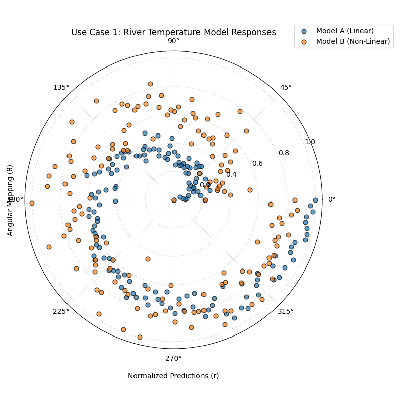
Two spirals of points, where the blue spiral (Linear Model) is tight and uniform, while the orange spiral (Non-Linear Model) is more dispersed and shows a different shape.

🧠 Analysis and Interpretation

This plot effectively contrasts the core behavior of the two models. Model A (blue) produces points that form a tight, consistent spiral. This visually confirms that its normalized predictions increase in a stable, linear fashion as the true temperature (angle) increases. In contrast, the points for Model B (orange) form a different pattern. Its spiral expands quickly at lower angles but then appears to compress at higher angles, visually revealing its non-linear response where predictions start to level off even as the true temperature continues to rise.

---

Use Case 2: Using Custom Angular Labels for Better Context

While mapping the angle to the true value is the default, the true value itself might not be the most intuitive label for the angular axis. For time series data, we often want to label the angle with the date or month. The z_values and z_label parameters are designed for exactly this.

Let’s analyze a 12-month forecast for a company’s monthly recurring revenue (MRR). We will map the true MRR to the angle for positioning, but we will label the angle with the month to make the plot easier to read.

# --- 1. Data Generation: Monthly Revenue Forecast ---
np.random.seed(42)
n_months = 12 * 5 # 5 years of monthly data
time_index = np.arange(n_months)
# A signal with growth and yearly seasonality
y_true_mrr = 100 + time_index * 2 + 20 * np.sin(time_index * 2 * np.pi / 12) + np.random.normal(0, 5, n_months)
y_pred_mrr = y_true_mrr + np.random.normal(0, 8, n_months)
# Our custom labels for the angular axis
month_labels = (time_index % 12) + 1

# --- 2. Plotting with Custom z_values ---
kd.plot_relationship(
    y_true_mrr,
    y_pred_mrr,
    names=["MRR Forecast"],
    title="Use Case 2: Revenue Forecast with Monthly Labels",
    acov="default",
    z_values=month_labels, # Provide the month numbers as labels
    z_label="Month of Year",
    s=30,
    savefig="gallery/images/gallery_plot_relationship_z_values.png"
)
plt.close()

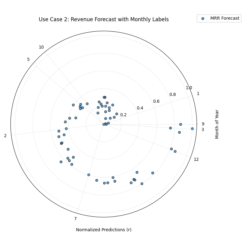
A spiral of points where the angular ticks are labeled with the month of the year (1-12) instead of the raw true value.

🧠 Interpretation

This plot is now much more interpretable for a time series analysis. Although the points are still positioned angularly based on the true MRR value, the angular tick labels now clearly show the month of the year. The z_label adds a title to these custom ticks. This allows us to diagnose seasonal patterns. For example, we could now easily see if the model’s performance (the tightness of the spiral) is worse during specific months, such as the end-of-year holiday season.

Best Practice

For time series or other sequentially ordered data, using z_values to label the angular axis with a time-based unit (like month, day, or hour) can make the plot vastly more intuitive and easier to interpret, providing richer context than the raw true values alone.

---

For a deeper understanding of the mathematical concepts behind the coordinate mapping and normalization, please refer back to the main True vs. Predicted Polar Relationship (plot_relationship()) section.

Conditional Quantile Bands

The plot_conditional_quantiles() function is a diagnostic for visualizing the conditional behavior of a probabilistic forecast. It answers the question: “How does my model’s entire predicted distribution, including its central tendency and uncertainty, change as a function of the true observed value?” It is the primary tool for visually diagnosing heteroscedasticity.

First, let’s break down the components of this detailed diagnostic plot.

Plot Anatomy

• Angle (θ): Represents the true observed value (\(y_{true}\)), sorted and mapped to the angular axis. The plot spirals outwards from the lowest true value to the highest.

• Radius (r): Represents the magnitude of the predicted value for each quantile.

• Central Line: The solid black line shows the median (Q50) forecast. Its spiral should ideally track the true value spiral (if it were plotted).

• Shaded Bands: Each shaded band represents a prediction interval (e.g., the 80% interval between Q10 and Q90). The width of these bands at any given angle visualizes the model’s predicted uncertainty for that specific true value.

Now, let’s apply this plot to a real-world problem where understanding conditional uncertainty is critical.

---

Use Case 1: Diagnosing Heteroscedasticity in Financial Forecasting

A core challenge in financial modeling is that volatility is not constant. A stock’s price may be stable and predictable during calm periods but highly volatile and uncertain during market turmoil. A good probabilistic model must capture this changing uncertainty.

Let’s simulate a forecast for an asset’s price, where the true volatility (and thus the model’s predictive uncertainty) increases as the asset’s price increases.

import kdiagram as kd
import numpy as np
import matplotlib.pyplot as plt

# --- 1. Data Generation: A forecast with heteroscedastic uncertainty ---
np.random.seed(0)
n_samples = 300
# True asset price, sorted to create a smooth spiral
y_true = np.linspace(50, 500, n_samples)
quantiles = np.array([0.1, 0.25, 0.5, 0.75, 0.9]) # For 80% and 50% intervals

# Key: Uncertainty (interval width) increases with the true value
error_std = 5 + (y_true / 500) * 40
# Generate quantile predictions based on this changing standard deviation
y_preds = np.zeros((n_samples, len(quantiles)))
y_preds[:, 2] = y_true + np.random.normal(0, 5, n_samples) # Median forecast
z_scores = np.array([-1.28, -0.67, 0, 0.67, 1.28]) # For 10,25,50,75,90
for i, z in enumerate(z_scores):
    y_preds[:, i] = y_preds[:, 2] + z * error_std

# --- 2. Plotting ---
kd.plot_conditional_quantiles(
    y_true, y_preds, quantiles,
    bands=[80, 50], # Show 80% and 50% intervals
    title="Use Case 1: Diagnosing Heteroscedasticity",
    savefig="gallery/images/gallery_conditional_quantiles_hetero.png"
)
plt.close()

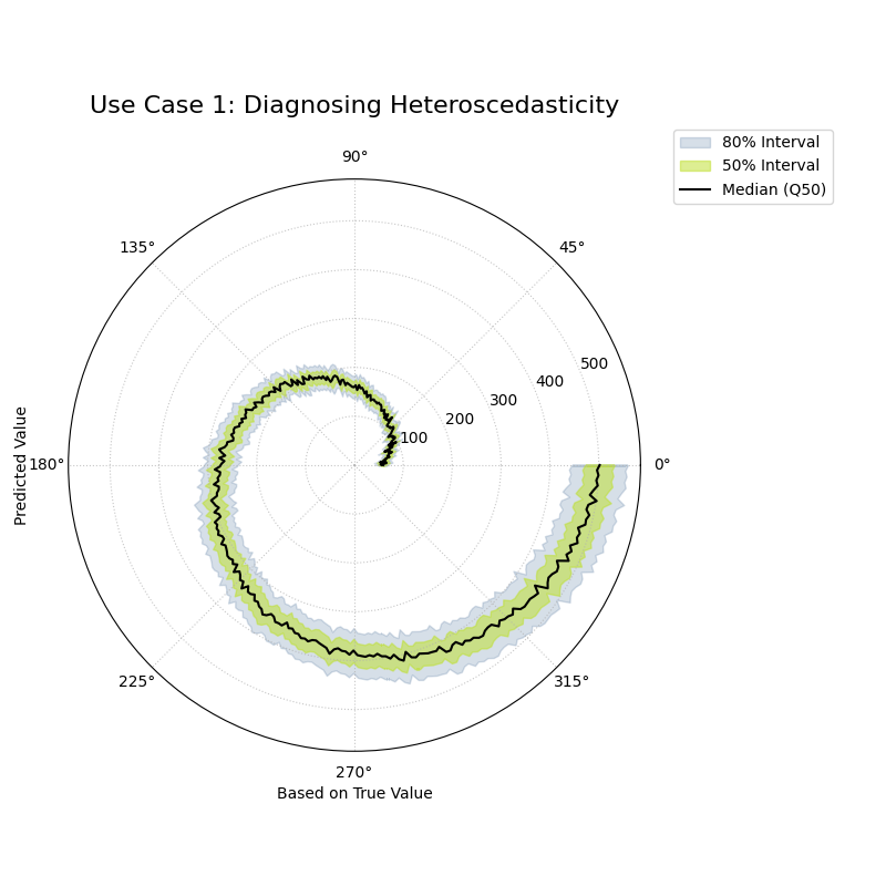
A spiral of quantile bands where the width of the bands clearly increases as the radius and angle increase, showing heteroscedasticity.

🧠 Analysis and Interpretation

This plot provides a clear and unambiguous diagnosis of the forecast’s uncertainty structure. The most important feature is the width of the shaded prediction intervals. The bands are very narrow at small angles (corresponding to low true asset prices) and become progressively wider as the spiral moves outwards towards higher true values. This is the classic visual signature of heteroscedasticity. It demonstrates that the model has correctly learned to be more uncertain (predicting a wider range of outcomes) when forecasting high asset prices, which are typically more volatile.

---

Use Case 2: Identifying a Homoscedastic (Naive) Model

To better appreciate a good heteroscedastic model, it’s useful to see what a naive, homoscedastic model looks like. This type of model incorrectly assumes that the level of uncertainty is constant, regardless of the situation.

Let’s create a forecast from a simpler model that uses a “one-size-fits-all” approach to uncertainty for the same financial asset.

# --- 1. Data Generation (uses y_true and quantiles from previous step) ---
# This model uses a constant, average uncertainty for all predictions
constant_error_std = 20.0
y_preds_homo = np.zeros((n_samples, len(quantiles)))
y_preds_homo[:, 2] = y_true + np.random.normal(0, 5, n_samples)
for i, z in enumerate(z_scores):
    y_preds_homo[:, i] = y_preds_homo[:, 2] + z * constant_error_std

# --- 2. Plotting ---
kd.plot_conditional_quantiles(
    y_true, y_preds_homo, quantiles,
    bands=[80, 50],
    cmap='magma',
    title="Use Case 2: A Naive (Homoscedastic) Forecast",
    savefig="gallery/images/gallery_conditional_quantiles_homo.png"
)
plt.close()

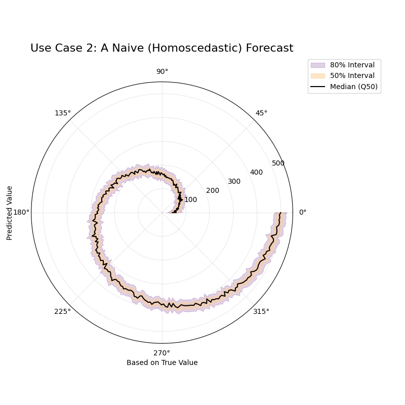
A spiral of quantile bands where the width of the shaded area remains constant from the center to the edge.

🧠 Interpretation

This plot shows a fundamentally different and more problematic behavior. The shaded bands now have a constant width as they spiral outwards. This demonstrates that the model is homoscedastic; it predicts the same level of uncertainty regardless of whether the true asset price is low or high. This is likely a flaw. The model will be underconfident (too wide) for low prices and dangerously overconfident (too narrow) for the more volatile high prices. This diagnostic clearly indicates that the model’s uncertainty estimates are too simplistic and unreliable for risk management.

See Also

The plot_credibility_bands() function provides a related but different view. While this plot shows how uncertainty changes with the true value, plot_credibility_bands (section Polar Credibility Bands) shows how the average uncertainty changes with a third, categorical feature (like the month of the year).

---

For a deeper understanding of the statistical concepts behind conditional distributions and heteroscedasticity, please refer back to the main Conditional Quantile Bands (plot_conditional_quantiles()) and section.

Error vs. True Value Relationship

The plot_error_relationship() function is a tool for going beyond simple error metrics and understanding the structure of a model’s errors. By plotting the forecast error against the true observed value, it helps answer a critical question: “Are my model’s errors correlated with the magnitude of the actual outcome?” Uncovering such a correlation is key to diagnosing conditional biases and other hidden flaws.

First, let’s break down the components of this diagnostic plot.

Plot Anatomy

• Angle (θ): Represents the true value (\(y_{true}\)), sorted and mapped to the angular axis. The plot spirals outwards as the true value increases. The angular labels are often hidden (mask_angle=True) as the progression is the key insight, not the specific values.

• Radius (r): Represents the forecast error or residual (\(e = y_{true} - y_{pred}\)). To handle positive and negative errors, the plot is shifted so that the radius represents the error relative to a “Zero Error” circle.

• Zero Error Circle: The dashed black circle is the crucial reference. Points falling on this line had a perfect prediction (error = 0). Points outside the circle are under-predictions (positive error), while points inside are over-predictions (negative error).

Now, let’s apply this diagnostic to a real-world problem to see how it can reveal different types of model deficiencies.

---

Use Case 1: Diagnosing a Conditional Bias

A common failure mode for regression models is a conditional bias, where the model is accurate for a certain range of values but becomes systematically biased for another.

Let’s simulate a model for predicting house prices that performs well on cheaper houses but consistently under-predicts the price of expensive luxury homes.

import kdiagram as kd
import numpy as np
import matplotlib.pyplot as plt

# --- 1. Data Generation: A model with conditional bias ---
np.random.seed(0)
n_samples = 250
# A skewed distribution of true house prices
y_true = np.random.lognormal(mean=12.5, sigma=0.5, size=n_samples)
# The model's error is proportional to the true value, causing under-prediction for high values
bias = y_true * 0.15
y_pred = y_true - bias + np.random.normal(0, 0.05 * y_true.max(), n_samples)

# --- 2. Plotting ---
kd.plot_error_relationship(
    y_true, y_pred,
    names=["House Price Model"],
    title="Use Case 1: Error vs. True Value (Conditional Bias)",
    s=40,
    mask_angle=True,
    savefig="gallery/images/gallery_error_relationship_bias.png"
)
plt.close()

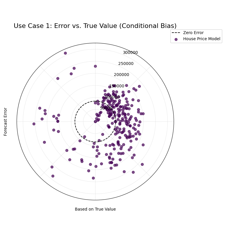
A spiral of error points that are centered on the zero-error line at small angles but drift progressively outwards at larger angles.

🧠 Analysis and Interpretation

This plot provides an immediate diagnosis of a serious model flaw. For low true values (small angles, near the plot’s start), the points are scattered symmetrically around the dashed “Zero Error” circle. However, as the true house price increases (as the spiral moves outwards), the entire cloud of error points systematically drifts outside the reference circle. This reveals a strong conditional bias: the model is accurate for low-priced homes but consistently under-predicts the value of high-priced homes, and the magnitude of this under-prediction grows with the price of the home.

---

Use Case 2: Diagnosing Heteroscedasticity

Another common issue is heteroscedasticity, where the variance of the model’s errors changes with the true value. The model might be very consistent for one range of outcomes but become erratic and unpredictable for another.

Let’s simulate a scientific instrument that is very precise when measuring small quantities but becomes much noisier and less reliable when measuring large quantities.

# --- 1. Data Generation: A model with heteroscedastic error ---
np.random.seed(42)
n_samples = 250
y_true_measurement = np.linspace(1, 100, n_samples)
# The standard deviation of the error increases with the true value
error_variance = y_true_measurement * 0.1
y_pred_measurement = y_true_measurement + np.random.normal(0, error_variance, n_samples)

# --- 2. Plotting ---
kd.plot_error_relationship(
    y_true_measurement, y_pred_measurement,
    names=["Instrument Model"],
    title="Use Case 2: Error vs. True Value (Heteroscedasticity)",
    s=40,
    savefig="gallery/images/gallery_error_relationship_hetero.png"
)
plt.close()

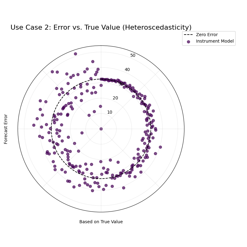
A spiral of error points that is very narrow at small angles but becomes progressively wider and more spread out at larger angles, forming a cone shape.

🧠 Interpretation

This plot reveals a different kind of problem. The cloud of error points remains centered on the “Zero Error” circle at all angles, indicating the model is unbiased. However, the vertical spread of the points (the width of the spiral) changes dramatically. It is very narrow for low true values (small angles) but “fans out,” becoming much wider for high true values. This is the classic signature of heteroscedasticity. It tells us that while the model is accurate on average, its predictions become far more inconsistent and unreliable when measuring larger quantities.

See Also

This plot is the direct companion to the plot_residual_relationship() function. This current plot answers - “Are my errors related to the **actual outcome*?”, while the ``plot_residual_relationship`` answers - *”Are my errors related to what my **model is predicting*?”* Both are crucial for a complete diagnosis of model residuals.

---

For a deeper understanding of the statistical concepts behind conditional bias and heteroscedasticity, please refer back to the main Error vs. True Value Relationship (plot_error_relationship()) section.

Residual vs. Predicted Relationship

The plot_residual_relationship() function provides a polar version of the classic residual plot, a fundamental diagnostic for any regression model. It is designed to answer the question: “Are my model’s errors correlated with its own predictions?” Uncovering such a pattern is key to diagnosing issues like heteroscedasticity and ensuring the model’s reliability across its full range of outputs.

First, let’s break down the components of this essential diagnostic plot.

Plot Anatomy

• Angle (θ): Represents the predicted value (\(y_{pred}\)), sorted and mapped to the angular axis. The plot spirals outwards as the predicted value increases.

• Radius (r): Represents the forecast error or residual (\(e = y_{true} - y_{pred}\)). The plot is shifted so that the radius represents the error relative to the “Zero Error” circle.

• Zero Error Circle: The dashed black circle is the reference line for a perfect prediction. Points outside the circle are under-predictions, while points inside are over-predictions.

Now, let’s apply this diagnostic to a real-world problem to see how it can reveal common model flaws.

---

Use Case 1: Diagnosing Heteroscedasticity

The most critical use of this plot is to check for heteroscedasticity, a condition where the variance of a model’s errors is not constant. A robust model should have errors that are equally spread out, regardless of the magnitude of its prediction.

Let’s simulate a model for predicting house prices that becomes more erratic and less reliable when it predicts higher prices.

import kdiagram as kd
import numpy as np
import matplotlib.pyplot as plt

# --- 1. Data Generation: A model with heteroscedastic errors ---
np.random.seed(42)
n_samples = 250
# A range of predicted house prices
y_pred = np.linspace(200000, 2500000, n_samples)
# Key: The error's standard deviation increases with the predicted price
error_variance = (y_pred / y_pred.max()) * 150000
errors = np.random.normal(0, error_variance, n_samples)
y_true = y_pred + errors

# --- 2. Plotting ---
kd.plot_residual_relationship(
    y_true, y_pred,
    names=["House Price Model"],
    title="Use Case 1: Diagnosing Heteroscedasticity",
    s=40,
    alpha=0.6,
    savefig="gallery/images/gallery_residual_relationship_hetero.png"
)
plt.close()

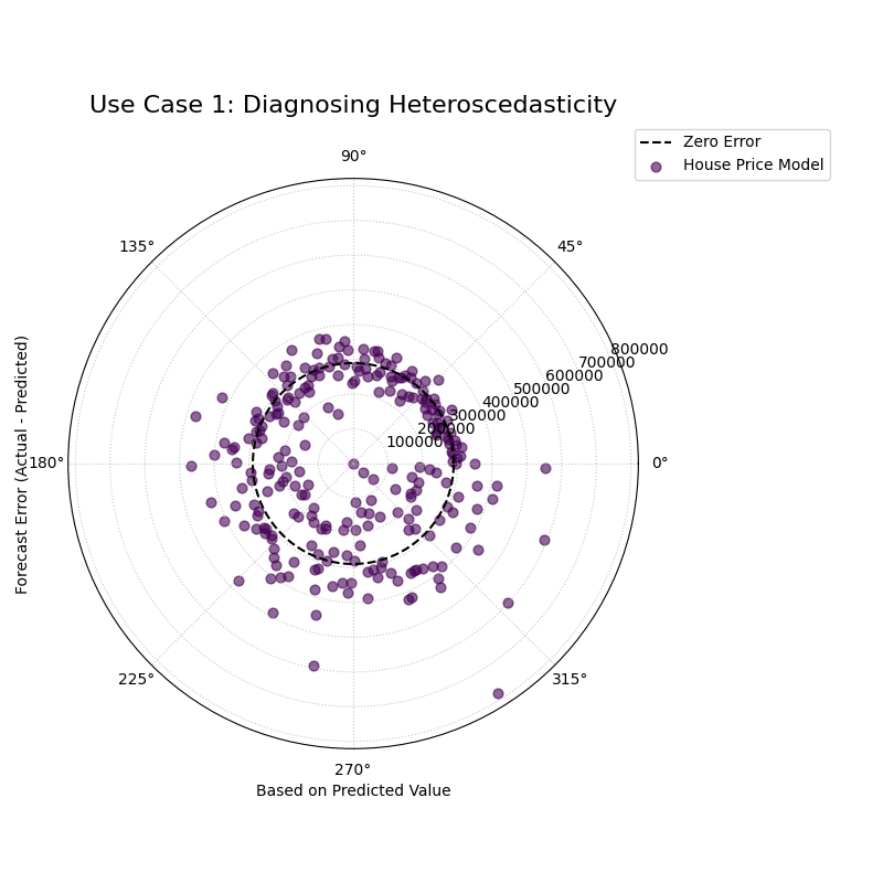
A spiral of error points that is very narrow for low predicted values but becomes progressively wider at higher predicted values, forming a distinct cone or fan shape.

🧠 Analysis and Interpretation

This plot reveals a classic and critical model flaw. While the error points remain centered on the dashed “Zero Error” circle (indicating the model is unbiased), their spread changes dramatically. The points are tightly clustered for low predicted values (small angles) but “fan out,” becoming much more widely scattered as the predicted price increases. This distinct cone shape is the unmistakable signature of heteroscedasticity. It tells us that the model’s reliability is not constant; it is precise and trustworthy for low-priced homes but becomes highly inconsistent and unreliable when predicting high prices.

---

Use Case 2: Identifying a Well-Behaved Model

To appreciate a flawed model, it helps to see what a good one looks like. A well-behaved model should produce residuals that are randomly and uniformly scattered around the zero-error line, forming a spiral of constant width.

Let’s simulate a second, improved house price model that has overcome the heteroscedasticity issue.

# --- 1. Data Generation: A homoscedastic (well-behaved) model ---
np.random.seed(0)
n_samples = 250
y_pred_good = np.linspace(200000, 2500000, n_samples)
# Key: The error's standard deviation is now constant
constant_error_variance = 80000
errors_good = np.random.normal(0, constant_error_variance, n_samples)
y_true_good = y_pred_good + errors_good

# --- 2. Plotting ---
kd.plot_residual_relationship(
    y_true_good, y_pred_good,
    names=["Improved Model"],
    title="Use Case 2: A Well-Behaved (Homoscedastic) Model",
    s=40,
    alpha=0.6,
    savefig="gallery/images/gallery_residual_relationship_good.png"
)
plt.close()

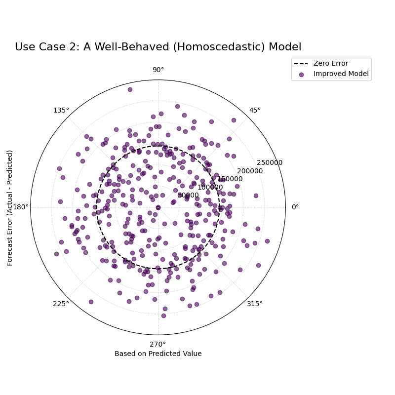
A spiral of error points that maintains a consistent width and is symmetrically scattered around the zero-error reference circle.

🧠 Interpretation

This plot is the signature of a well-behaved, homoscedastic model. The points form a spiral of constant width, and they are randomly and symmetrically scattered around the “Zero Error” circle at all angles (all prediction levels). This indicates that the variance of the model’s errors is independent of the magnitude of its predictions. This is the ideal, textbook result for a residual plot and gives us confidence that the model is reliable across its entire operational range.

See Also

This plot is the direct companion to the plot_error_relationship() function. The plot_error_relationship answers: “Are my errors related to the **actual outcome*?” while plot_residual_relationship() answers: “Are my errors related to what my **model is predicting*?”* Both are crucial for a complete diagnosis of model residuals.

---

For a deeper understanding of the statistical assumptions behind residual analysis, please refer back to the main Residual vs. Predicted Relationship (plot_residual_relationship()) section.

Practical Application: Regression Diagnosis

While the previous examples showcase each function individually, their true analytical power is unleashed when used together in a structured workflow. A robust model evaluation goes beyond a single plot; it involves a systematic investigation from multiple angles to build a complete picture of a model’s behavior.

This case study will walk you through a realistic, multi-step analysis, demonstrating how the plots from the relationship module can be combined into a single, comprehensive diagnostic dashboard to solve a complex modeling problem.

Case Study: Modeling Corporate Growth

The Business Problem: An investment firm wants to model the relationship between a company’s annual R&D spending and its subsequent revenue growth. Understanding this relationship is key to identifying high-potential investment opportunities.

The Models: The data science team has developed two competing models:

1. “Linear Model”: A simple, interpretable model assuming a straightforward, linear link between R&D and growth.

2. “ML Model”: A more complex machine learning model (e.g., Gradient Boosting) capable of learning non-linear patterns and providing probabilistic forecasts.

The Core Questions: The firm needs a deep understanding of these models before deploying them:

1. What is the fundamental response pattern of each model? Does the ML model’s non-linearity seem plausible?

2. How does the ML model’s uncertainty change? Does it correctly predict more uncertainty for high-growth companies?

3. Do the models suffer from hidden biases? For instance, do they systematically misjudge companies with very high or very low R&D spending?

Let’s use k-diagram to create a 2x2 diagnostic dashboard to answer all these questions at once.

Practical Example

import kdiagram as kd
import pandas as pd
import numpy as np
import matplotlib.pyplot as plt

# --- 1. Data Generation: R&D Spending vs. Revenue Growth ---
np.random.seed(42)
n_companies = 250
# True R&D spending (our feature)
rd_spending = np.linspace(1, 20, n_companies)
# True revenue growth has a non-linear, saturating relationship with R&D
true_growth = 50 - 45 * np.exp(-0.15 * rd_spending) + np.random.normal(0, 1.5, n_companies)

# --- 2. Generate Predictions for Both Models ---
# Linear Model: A simple straight-line fit
linear_pred = 2.0 * rd_spending + 5 + np.random.normal(0, 3, n_companies)
# ML Model: A better non-linear fit
ml_pred = true_growth + np.random.normal(0, 2, n_companies)

# Probabilistic forecast from the ML Model (heteroscedastic)
quantiles = np.array([0.1, 0.25, 0.5, 0.75, 0.9])
error_std = 1.5 + (true_growth / true_growth.max()) * 5
z_scores = np.array([-1.28, -0.67, 0, 0.67, 1.28])
ml_quantiles = ml_pred[:, np.newaxis] + z_scores * error_std[:, np.newaxis]

# --- 3. Create a 2x2 Figure for our Diagnostic Dashboard ---
fig = plt.figure(figsize=(18, 18))
ax1 = fig.add_subplot(2, 2, 1, projection='polar')
ax2 = fig.add_subplot(2, 2, 2, projection='polar')
ax3 = fig.add_subplot(2, 2, 3, projection='polar')
ax4 = fig.add_subplot(2, 2, 4, projection='polar')

# --- 4. Populate the Dashboard with Diagnostics ---
# Panel A: High-Level Relationship Comparison
kd.plot_relationship(
    true_growth, linear_pred, ml_pred, ax=ax1,
    names=["Linear Model", "ML Model"],
    title='(A) Model Response Patterns'
)
# Panel B: Conditional Uncertainty of the ML Model
kd.plot_conditional_quantiles(
    true_growth, ml_quantiles, quantiles, ax=ax2,
    bands=[80, 50],
    title='(B) ML Model Conditional Uncertainty',
    cmap="tab10"
)
# Panel C: Error vs. True Value (Conditional Bias Check)
kd.plot_error_relationship(
    true_growth, linear_pred, ml_pred, ax=ax3,
    names=["Linear Model", "ML Model"],
    title='(C) Error vs. True Growth (Bias)',
    cmap="tab10"
)
# Panel D: Residual vs. Predicted Value (Heteroscedasticity Check)
kd.plot_residual_relationship(
    true_growth, linear_pred, ml_pred, ax=ax4,
    names=["Linear Model", "ML Model"],
    title='(D) Residual vs. Predicted Growth (Variance)',
    cmap="tab10"
)

fig.suptitle('Comprehensive Regression Diagnostic Dashboard', fontsize=20)
fig.tight_layout(rect=[0, 0.03, 1, 0.96])
fig.savefig("gallery/images/gallery_relationship_dashboard.png")
plt.close(fig)

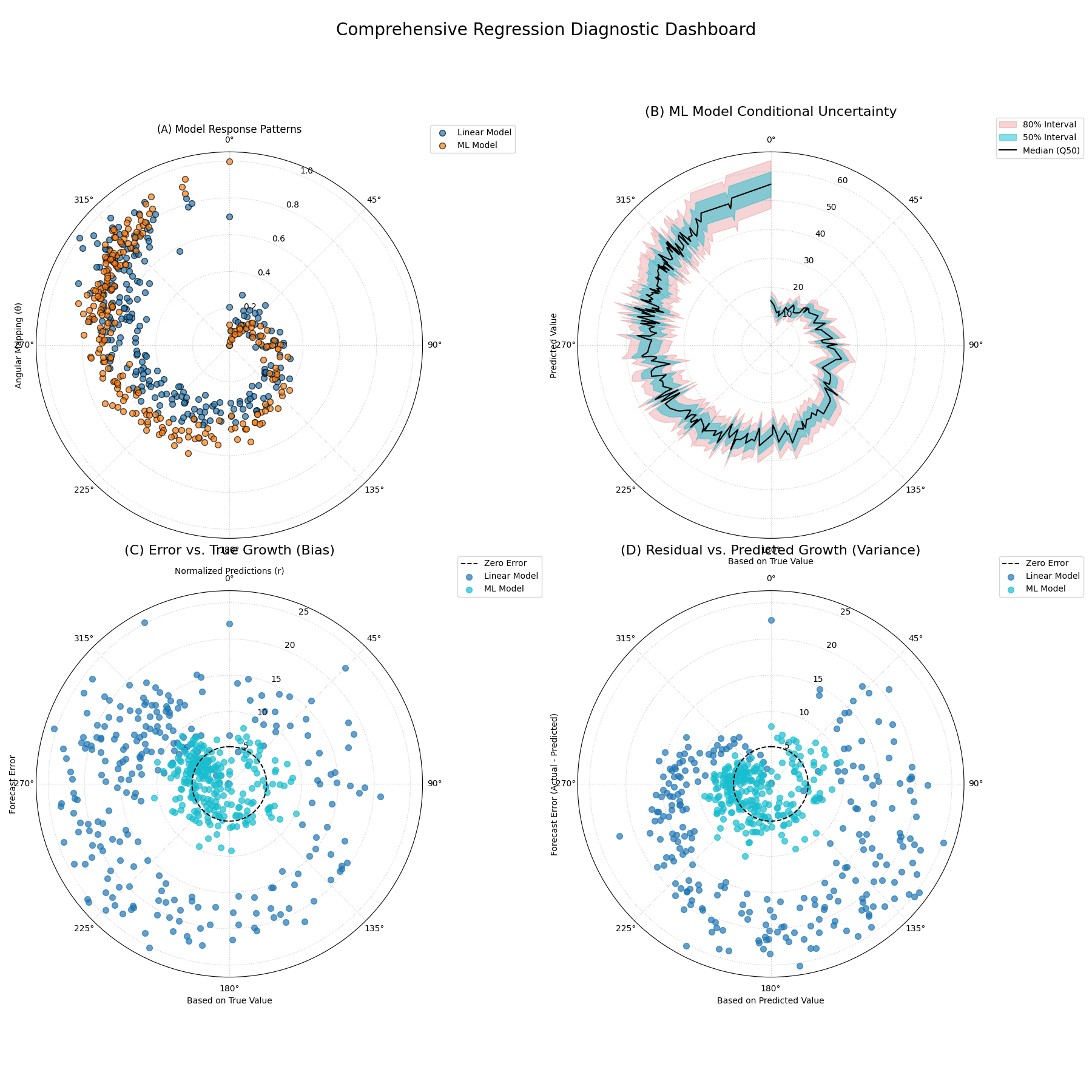
A comprehensive four-panel diagnostic plot comparing a linear and an ML model, showing their response patterns, uncertainty structures, and error characteristics.

🧠 Analysis and Interpretation

This diagnostic dashboard provides a complete story, with each panel building on the last to deliver a rich and nuanced verdict on the two models.

Panel A (Model Response Patterns): This high-level view immediately shows the difference in the models’ fundamental behavior. The Linear Model (blue) forms a perfect, uniform spiral, confirming its simple straight-line assumption. In contrast, the ML Model (orange) forms a spiral that is compressed at higher angles (higher growth), correctly capturing the non-linear, saturating nature of the true data. This suggests the ML model is a better fit.

Panel B (Conditional Uncertainty): Focusing on the ML model, this plot reveals how its uncertainty changes. The shaded quantile bands are narrow at low growth values (near the center) and become progressively wider as the true growth increases. This is a sign of a sophisticated model that has learned to be heteroscedastic—it correctly predicts higher uncertainty for the high-growth companies that are inherently more volatile.

Panel C (Error vs. True Growth): This plot diagnoses conditional bias. The ML model’s errors (cyan) are symmetrically scattered around the “Zero Error” circle at all angles, confirming it is unbiased. The Linear Model’s errors (blue), however, show a systematic drift. They start inside the circle (over-prediction for low growth) and end up far outside it (severe under-prediction for high growth). This confirms the Linear Model is fundamentally misspecified.

Panel D (Residual vs. Predicted Growth): This final check confirms our findings. The ML model’s residuals (cyan) show a constant, random scatter, indicating its error variance is well-behaved. The Linear Model’s residuals (blue) show a clear “frowning face” pattern, a classic sign of a misspecified model struggling to fit a non-linear relationship.

Overall Conclusion: The dashboard provides overwhelming evidence that the ML Model is superior in every aspect. It not only fits the data better but also provides a realistic, heteroscedastic uncertainty estimate and produces well-behaved, unbiased residuals, making it a far more trustworthy tool for investment decisions.

---

For a deeper understanding of the statistical concepts behind these advanced regression diagnostics, please refer back to the main Visualizing Relationships section.