Uncertainty Visualizations

This page showcases examples of plots specifically designed for exploring, diagnosing, and communicating aspects of predictive uncertainty using k-diagram.

Note

You need to run the code snippets locally to generate the plot images referenced below (e.g., ../images/gallery_actual_vs_predicted.png). Ensure the image paths in the .. image:: directives match where you save the plots (likely an images subdirectory relative to this file, e.g., ../images/).

Actual vs. Predicted

The plot_actual_vs_predicted() function is the foundational tool for forecast evaluation. It creates a direct, point-by-point comparison of observed outcomes against a model’s central prediction, providing an immediate and intuitive assessment of accuracy and bias.

Before diving into complex diagnostics, it is essential to master the anatomy of this plot.

Plot Anatomy

• Angle (θ): Represents the sample’s position in the dataset, arranged sequentially around the circle. If a theta_col is provided in a future version, it could represent an explicit ordering variable like time or a spatial coordinate.

• Radius (r): Directly corresponds to the magnitude of the value. Both the actual_col and pred_col are plotted on this axis, allowing for a direct comparison of their magnitudes at each angular position.

• Azimuth: The azimuth (the circular path at a constant radius) does not represent a specific metric itself, but tracing it helps in comparing how predictions and actuals change relative to each other across the dataset.

Now, let’s explore how to apply this plot to a real-world scenario, progressing from a basic check to a more advanced, customized visualization.

---

Use Case 1: A Basic “Sanity Check”

The most fundamental use of this plot is as a “sanity check” for a single model. After training, you need an immediate visual answer to the question: “Is my model’s forecast even in the right ballpark?” By plotting the predictions as points against the true values, we can get a quick, high-level sense of the model’s performance.

import kdiagram as kd
import pandas as pd
import numpy as np
import matplotlib.pyplot as plt

# --- 1. Data Generation ---
# Simulate a cyclical signal (e.g., seasonal sales) with some noise
np.random.seed(66)
n_points = 120
signal = 20 + 15 * np.cos(np.linspace(0, 6 * np.pi, n_points))
df_basic = pd.DataFrame({
    'actual_sales': signal + np.random.randn(n_points) * 3,
    'predicted_sales': signal * 0.9 + np.random.randn(n_points) * 2 + 2
})

# --- 2. Plotting with Dots ---
kd.plot_actual_vs_predicted(
    df=df_basic,
    actual_col='actual_sales',
    pred_col='predicted_sales',
    title='Use Case 1: Basic Sanity Check (Dots)',
    line=False, # Use dots for a point-by-point view
    r_label="Sales Volume",
    actual_props={'s': 30, 'alpha': 0.8, 'color':'black'},
    pred_props={'s': 40, 'marker': 'x', 'alpha': 0.8, 'color':'#E53E3E'}, # Red 'x'
    savefig="gallery/images/gallery_avp_basic.png"
)

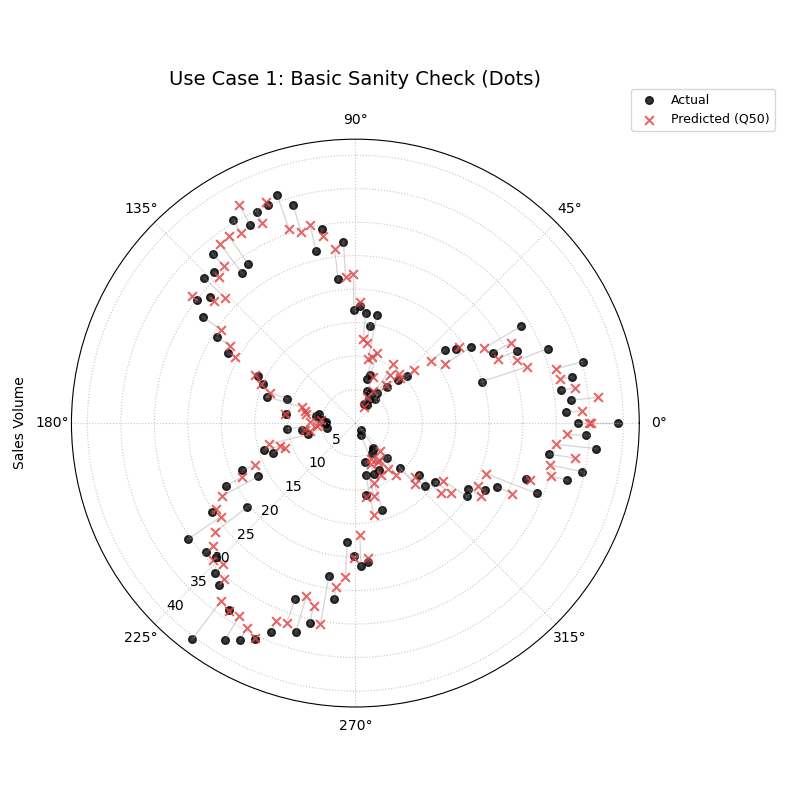
A point-by-point comparison where black dots represent actual sales and red crosses represent the model’s predictions.

🧠 Analysis and Interpretation

This plot provides a direct, sample-by-sample comparison. The black dots (actuals) and red crosses (predictions) form clear cyclical patterns, indicating the model has successfully captured the main seasonal trend. We can see that the predictions generally track the actual values, but with some scatter. In some areas, particularly at the peaks of the cycle (outer radius), the red crosses appear to be systematically inside the cloud of black dots, hinting at a potential under-prediction bias. This initial check confirms the model is reasonable but warrants a closer look.

---

Use Case 2: Comparing Competing Models with Lines

A more advanced and common task is to compare the performance of two or more competing models. By plotting their predictions as continuous lines, we can better visualize and contrast their tracking behavior and systemic biases.

Let’s imagine we have our original model (“Biased Model”) and a new, improved model (“Tracking Model”). We want to see if the new model corrects the under-prediction bias we suspected in the first use case.

# --- 1. Add a second model's prediction to our DataFrame ---
# (Assumes df_basic from the previous step is available)
df_multi = df_basic.copy()
df_multi['tracking_model'] = df_multi['actual_sales'] + np.random.normal(0, 1.5, n_points)
df_multi.rename(columns={'predicted_sales': 'biased_model'}, inplace=True)

# --- 2. Plotting with Lines for Comparison ---
# Note: This function is designed for one prediction column. To compare
# multiple, we would typically call it multiple times on the same axes
# or use a different plot. For this example, we will create two separate plots.
# (This is a good place to show how to use the function twice if needed)

fig, (ax1, ax2) = plt.subplots(1, 2, figsize=(16, 8),
                             subplot_kw={'projection': 'polar'})

# after creating ax1, ax2, let extend re-position r default
for a in (ax1, ax2):
    a.set_ylabel(None)
    a.set_rlabel_position(225)

# Plot for the Biased Model
kd.plot_actual_vs_predicted(
    df=df_multi,
    actual_col='actual_sales',
    pred_col='biased_model',
    title='Biased Model Performance',
    show_legend=False,
    ax= ax1
)
ax1.set_ylabel("Sales Volume", labelpad=32)

# Plot for the Tracking Model
ax2 = kd.plot_actual_vs_predicted(
    df=df_multi,
    actual_col='actual_sales',
    pred_col='tracking_model',
    title='Improved Tracking Model Performance',
    pred_props={'color': '#38A169'}, # Green for the good model
    ax= ax2
)
ax2.set_ylabel("Sales Volume", labelpad=32)

fig.suptitle('Use Case 2: Comparing Competing Models', fontsize=16)
kd.savefig("gallery/images/gallery_avp_multi.png")
plt.close(fig)

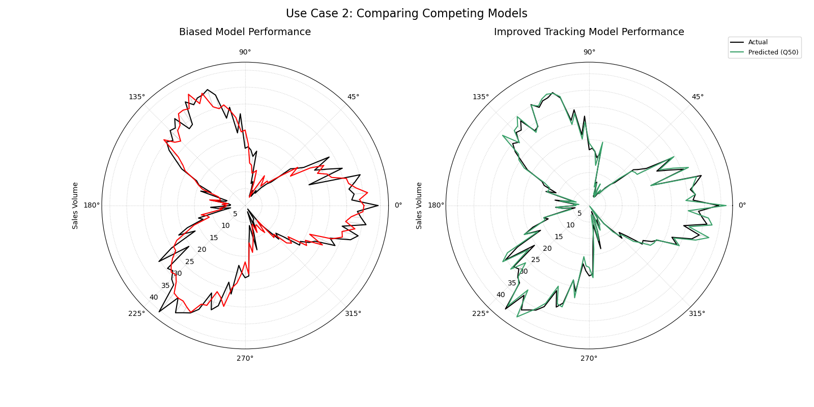
Side-by-side comparison. The left plot shows a biased model with a prediction line that does not fully match the actuals. The right plot shows an improved model where the lines overlap almost perfectly.

🧠 Interpretation

The side-by-side comparison makes the performance difference crystal clear. The Biased Model (left) shows a red prediction spiral that is visibly smoother and has a smaller amplitude than the black actuals spiral, confirming a systematic under-prediction bias at the peaks. In contrast, the Improved Tracking Model (right) shows a green prediction spiral that almost perfectly overlays the black actuals spiral, demonstrating its superior accuracy and lack of significant bias.

---

Use Case 3: Focused Analysis with Custom Styling

Sometimes, you need to create a presentation-ready plot that focuses on a specific segment of your data, such as a critical business season. By using the acov (angular coverage) parameter and customizing the plot properties, we can create a more targeted and visually polished diagnostic.

Let’s focus on the first half of our sales cycle using a half-circle layout to make the details easier to see.

# --- 1. Use the multi-model DataFrame from the previous step ---
# (Assumes df_multi is available, i.e from the previous step)

# --- 2. Create a focused and styled plot ---
kd.plot_actual_vs_predicted(
    df=df_multi.head(60), # Focus on the first half of the cycle
    actual_col='actual_sales',
    pred_col='tracking_model',
    acov='half_circle', # Use a 180-degree layout
    title='Use Case 3: Focused Analysis (First 60 Samples)',
    r_label="Sales Volume",
    actual_props={'color': '#2D3748', 'linewidth': 2.5, 'label': 'Actual Sales'},
    pred_props={'color': '#38A169', 'linewidth': 2.5, 'linestyle': '--', 'label': 'Forecast'},
    savefig="gallery/images/gallery_avp_focused.png"
)

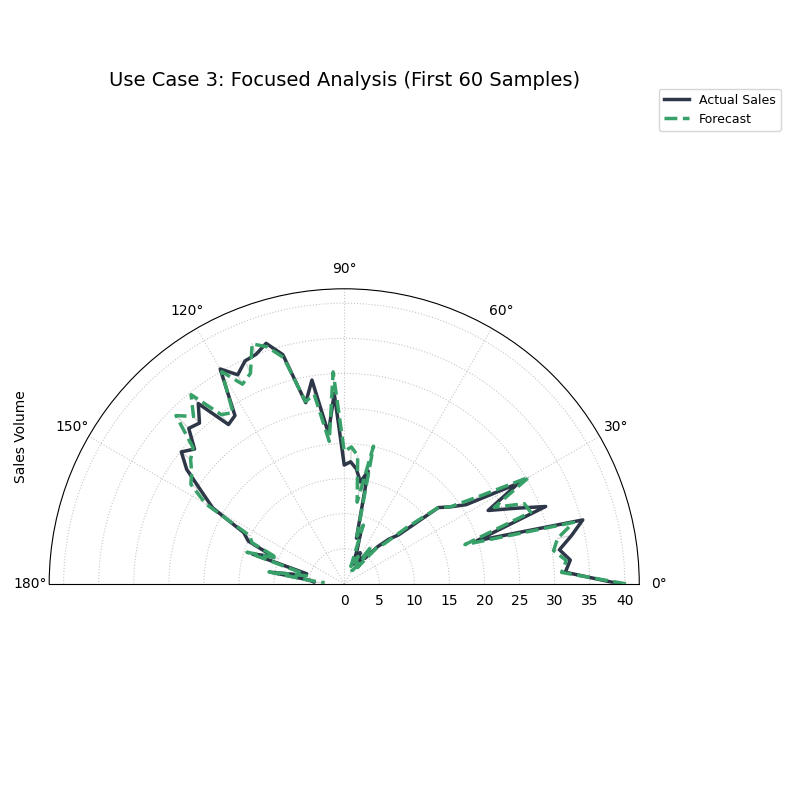
A styled, half-circle plot focusing on a specific period, with thicker, custom-colored lines for better presentation.

🧠 Interpretation

By limiting the angular coverage to a half-circle and using only the first 60 data points, the plot becomes less cluttered and easier to inspect in detail. The custom styling—using thicker, dashed, and differently colored lines—enhances its readability, making it ideal for inclusion in a report or presentation. This focused view reaffirms the excellent tracking performance of the improved model during this specific period.

---

For a deeper understanding of the mathematical concepts behind the plot, you may refer to the main Actual vs. Predicted Comparison (plot_actual_vs_predicted()) section.

Anomaly Magnitude

The plot_anomaly_magnitude() function is a specialized diagnostic tool that focuses exclusively on forecast failures. It filters out all successful predictions and creates a polar scatter plot of only the “anomalies”—cases where the true value fell outside the predicted uncertainty interval. This allows for a detailed investigation into the location, type, and severity of a model’s most significant errors.

First, let’s understand the key components of this specialized plot.

Plot Anatomy

• Angle (θ): Represents the sample’s position in the dataset. By default, it is based on the DataFrame index, but if theta_col is provided, the points are ordered according to that column’s values. This can reveal if failures are clustered in time or space.

• Radius (r): Directly corresponds to the severity of the anomaly, calculated as the absolute distance from the true value to the prediction interval boundary that was breached (\(|y_{actual} - y_{bound}|\)). Points far from the center represent critical failures.

• Color: Distinguishes the type of anomaly. The plot uses separate colormaps (cmap_over and cmap_under) to instantly differentiate between over-predictions (e.g., actual > Q90) and under-predictions (e.g., actual < Q10).

Now, let’s apply this diagnostic to a few real-world scenarios to see how it can be used to generate critical insights.

---

Use Case 1: Balanced Anomalies in Financial Forecasting

In many forecasting problems, we expect anomalies to be somewhat symmetrical. For a well-calibrated model predicting stock returns, for instance, the number and magnitude of unexpectedly large gains (over- predictions) should be similar to the number and magnitude of unexpectedly large losses (under-predictions). This first example simulates such a balanced scenario.

import kdiagram as kd
import pandas as pd
import numpy as np
import matplotlib.pyplot as plt

# --- 1. Data Generation: Balanced Anomalies ---
np.random.seed(42)
n_points = 200
df = pd.DataFrame({'trading_day': range(n_points)})
df['actual_return'] = np.random.normal(loc=0, scale=1.5, size=n_points)
# A well-calibrated 80% interval
df['q10'] = -1.28 * 1.5
df['q90'] = 1.28 * 1.5
# Manually add some large, symmetric anomalies
anomaly_indices = np.random.choice(n_points, 40, replace=False)
df.loc[anomaly_indices, 'actual_return'] = np.random.choice([-1, 1], 40) * np.random.uniform(2.5, 5, 40)

# --- 2. Plotting ---
kd.plot_anomaly_magnitude(
    df=df,
    actual_col='actual_return',
    q_cols=['q10', 'q90'],
    title='Use Case 1: Balanced Financial Return Anomalies',
    cbar=True,
    s=40,
    verbose=0,
    savefig="gallery/images/gallery_anomaly_magnitude_balanced.png"
)

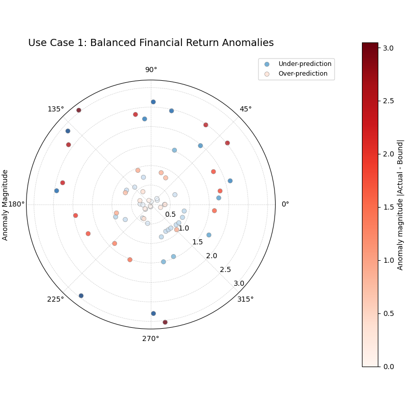
A balanced set of anomalies, with roughly equal numbers of over-predictions (red) and under-predictions (blue) distributed at various magnitudes.

🧠 Analysis and Interpretation

This plot reveals that the model’s interval failures are balanced. There are roughly equal numbers of over-predictions (red dots, where the actual return was higher than the predicted maximum) and under-predictions (blue dots, where the actual return was lower than the predicted minimum). The magnitudes (radii) of these failures are also fairly symmetrical. This is the signature of a model whose uncertainty is unbiased, even if the number of anomalies (40 out of 200, or 20%) is exactly what you would expect from an 80% prediction interval.

---

Use Case 2: Asymmetric Risk in Supply Chain Management

Not all anomalies are created equal. In many business contexts, one type of error is far more costly than the other. This plot is an excellent tool for diagnosing such asymmetric risks.

Consider a model forecasting the arrival time of shipments. A shipment arriving a day early (an under-prediction) is a minor inconvenience. A shipment arriving a day late (an over-prediction) can halt a production line and be extremely costly. We need to check if our model is prone to the more dangerous type of error.

# --- 1. Data Generation: Asymmetric Anomalies ---
np.random.seed(0)
n_points = 200
df_shipping = pd.DataFrame({'shipment_id': range(n_points)})
df_shipping['actual_arrival_day'] = np.random.uniform(5, 10, n_points)
df_shipping['q10_arrival'] = df_shipping['actual_arrival_day'] - 1
df_shipping['q90_arrival'] = df_shipping['actual_arrival_day'] + 1
# Manually add mostly LATE arrivals (over-predictions)
late_indices = np.random.choice(n_points, 35, replace=False)
early_indices = np.random.choice(list(set(range(n_points)) - set(late_indices)), 5, replace=False)
df_shipping.loc[late_indices, 'actual_arrival_day'] += np.random.uniform(1.5, 4, 35)
df_shipping.loc[early_indices, 'actual_arrival_day'] -= np.random.uniform(1.5, 4, 5)

# --- 2. Plotting ---
kd.plot_anomaly_magnitude(
    df=df_shipping,
    actual_col='actual_arrival_day',
    q_cols=['q10_arrival', 'q90_arrival'],
    title='Use Case 2: Asymmetric Risk in Shipping Forecasts',
    cbar=True,
    s=40,
    verbose=0,
    savefig="gallery/images/gallery_anomaly_magnitude_asymmetric.png"
)

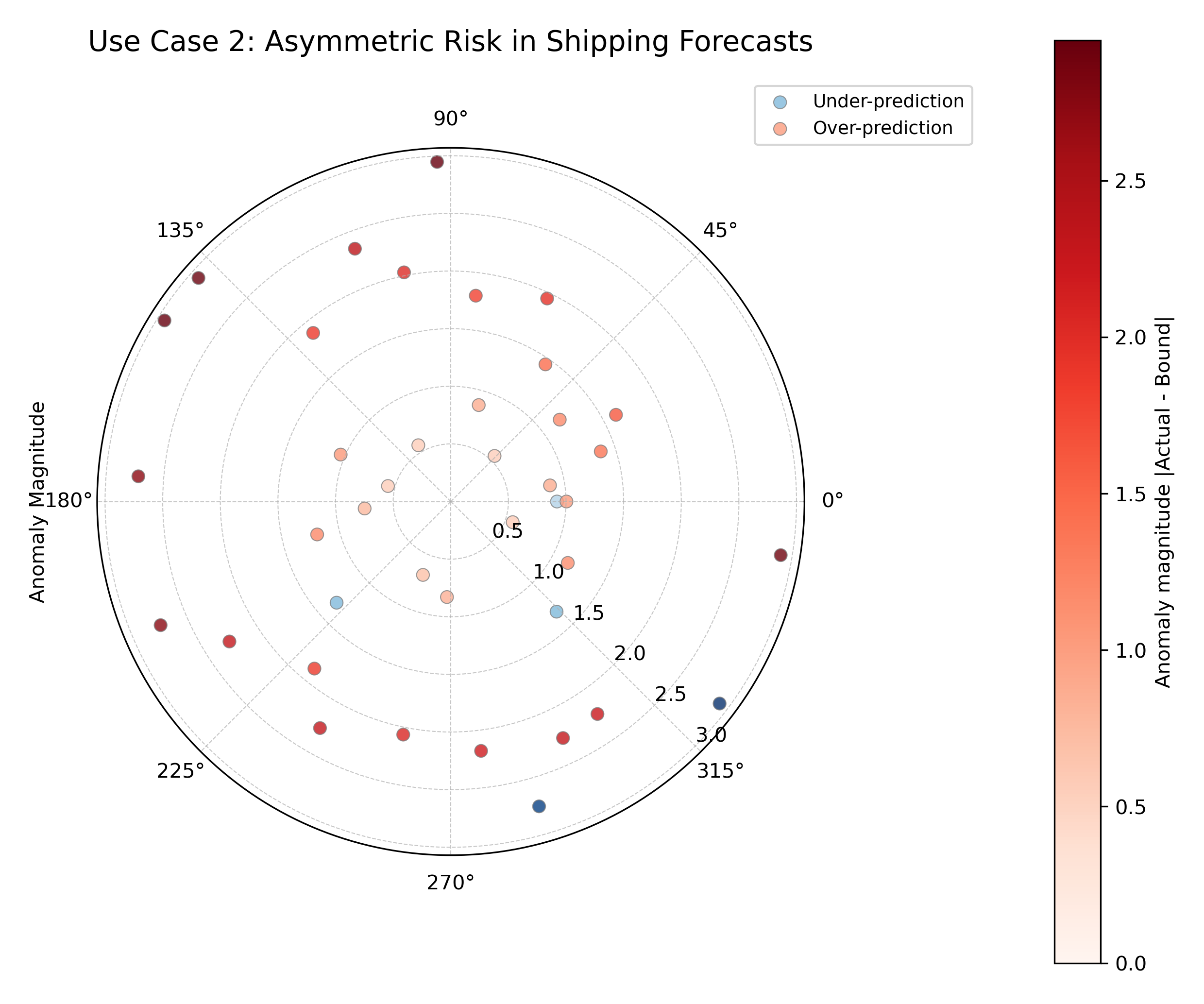
An asymmetric distribution of anomalies, where costly late arrivals (red dots) are far more frequent and severe than early arrivals (blue dots).

🧠 Interpretation

This plot immediately reveals a critical flaw in the forecasting model. The anomalies are overwhelmingly red, indicating that when the model fails, it is almost always because the shipment arrived later than the predicted window. Furthermore, several of these red points are at a large radius, indicating severe delays of 3-4 days. This plot provides a clear, data-driven warning that the model is too optimistic and exposes the company to significant risk from late shipments.

---

For an understanding of the mathematical concepts behind the plot, you may refer to the main Anomaly Magnitude Analysis (plot_anomaly_magnitude()) section.

Overall Coverage

The plot_coverage() function provides a high-level summary of a model’s reliability. It calculates the empirical coverage rate—the percentage of times the true value actually falls within a model’s predicted interval—and visualizes this score for one or more models, making it an essential first-pass check for forecast calibration.

Before we explore its use, let’s break down the anatomy of its most distinct visualization: the radar plot.

Plot Anatomy (Radar Chart)

• Angle (θ): Each angular sector is assigned to a different model or prediction set provided to the function.

• Radius (r): Directly corresponds to the calculated coverage score, ranging from 0 at the center to 1 (100%) at the outer edge.

• Azimuth: The azimuth, or the circular path, represents a line of constant coverage. The plot’s grid lines are drawn at specific coverage levels (e.g., 0.2, 0.4, 0.6, 0.8) to serve as a reference.

With this in mind, let’s walk through several real-world scenarios to see how this function can be applied.

---

Use Case 1: Basic Comparison with a Bar Chart

The simplest way to compare the overall coverage of a few models is with a standard bar chart. It provides a clean, straightforward view of the final scores.

Let’s imagine a financial analyst is comparing two models that predict an 80% confidence interval for a stock’s daily return. They need a quick, unambiguous visualization to see which model’s interval is more reliable.

import kdiagram as kd
import numpy as np
import matplotlib.pyplot as plt

# --- 1. Data Generation ---
np.random.seed(42)
n = 200
y_true = np.random.normal(0.0, 1.0, size=n)
q_levels = [0.10, 0.90]
z80 = 1.28155
sigma_mu = 1.0 # Assume model's error std dev
mu = y_true + np.random.normal(0.0, sigma_mu, size=n)

# Model A: calibrated -> predicted std matches error std
s_pred_A = sigma_mu
q10_A = mu - z80 * s_pred_A
q90_A = mu + z80 * s_pred_A
y_pred_A = np.stack([q10_A, q90_A], axis=1)

# Model B: over-confident -> predicted std is too small
s_pred_B = 0.5 * sigma_mu
q10_B = mu - z80 * s_pred_B
q90_B = mu + z80 * s_pred_B
y_pred_B = np.stack([q10_B, q90_B], axis=1)

# --- 2. Plotting with kind='bar' ---
kd.plot_coverage(
    y_true,
    y_pred_A,
    y_pred_B,
    names=['Model A (Calibrated)', 'Model B (Over-Confident)'],
    q=q_levels,
    kind='bar',
    title='Use Case 1: Basic Coverage Comparison (Bar Chart)',
    verbose=0,
)
kd.savefig("gallery/images/gallery_coverage_bar.png")

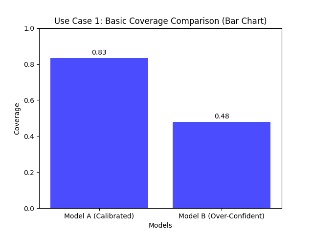
A simple bar chart comparing the empirical coverage of two models against the nominal 80% rate.

🧠 Analysis and Interpretation

This bar chart provides a clear and immediate result for the 80% nominal interval. Model A achieves a coverage of 83%, which is very close to the 80% target, indicating it is well-calibrated. In contrast, Model B has a much lower coverage of 48%, revealing that it is severely over-confident—its prediction intervals are far too narrow and fail to capture the true outcome more than half the time. For a reliable forecast, Model A is the clear choice.

---

Use Case 2: Multi-Model Profile with a Radar Chart

When comparing three or more models, a radar chart can provide a more holistic “profile” view. It’s particularly effective for showing how different models perform relative to the ideal 100% coverage limit and to each other.

Let’s expand our analysis to include a third model that is under-confident (its intervals are too wide).

# --- 1. Data Generation (assumes previous data is available) ---
# Model C (under-confident -> intervals are too wide)
s_pred_C = 1.5 * sigma_mu
q10_C = mu - z80 * s_pred_C
q90_C = mu + z80 * s_pred_C
y_pred_C = np.stack([q10_C, q90_C], axis=1)

# --- 2. Plotting with kind='radar' ---
kd.plot_coverage(
    y_true,
    y_pred_A,
    y_pred_B,
    y_pred_C,
    names=['A (Calibrated)', 'B (Over-Confident)', 'C (Under-Confident)'],
    q=q_levels,
    kind='radar',
    cov_fill=True,
    radar_fill_alpha=0.3,
    title='Use Case 2: Multi-Model Coverage Profile (Radar)',
    verbose=0,
    savefig="gallery/images/gallery_coverage_radar_multi.png"
)

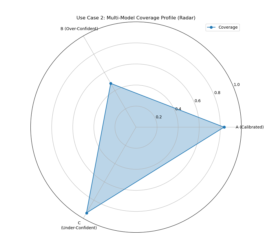
A radar chart comparing three models, showing one well-calibrated, one over-confident (low score), and one under-confident (high score).

🧠 Interpretation

The radar chart creates a “fingerprint” of the models’ reliability. The point for Model A lies near the 0.8 radial grid line, matching the 80% target well. The point for Model B collapses towards the center, showing its low coverage and confirming it is over-confident. Conversely, the point for Model C is pushed far out towards the 1.0 boundary, clearly visualizing its under-confidence and excessively wide intervals.

---

Use Case 3: Single-Model Focus with Gradient Fill

When you want to focus on the performance of a single, primary model, the radar plot with cov_fill=True creates a special visualization with a radial gradient. This provides a visually appealing way to show a single score against the [0, 1] scale.

Let’s create a presentation-ready plot for our best model, Model A.

# --- 1. Use the well-calibrated Model A from the previous step ---

# --- 2. Plotting a single model with gradient fill ---
kd.plot_coverage(
    y_true,
    y_pred_A,
    names=['Model A (Calibrated)'],
    q=q_levels,
    kind='radar',
    cov_fill=True, # Activate special single-model fill
    cmap='Greens',
    title='Use Case 3: Single-Model Coverage Report',
    verbose=0,
    savefig="gallery/images/gallery_coverage_radar_single.png"
)

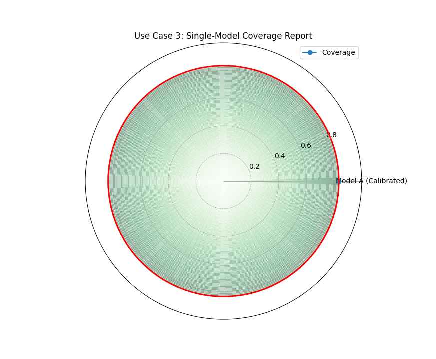
A focused view of a single model’s coverage, where a radial gradient fills up to the calculated score, marked by a solid red circle.

🧠 Interpretation

This focused view is excellent for reports. The green radial gradient fills the polar area up to the model’s calculated coverage score, which is marked by the solid red circle. The concentric gray grid lines provide a clear scale. In this case, we can see the red circle sits very close to the 0.8 grid line, providing a visually unmistakable confirmation that the model is well-calibrated against its 80% nominal target.

---

For a deeper understanding of the statistical concepts behind coverage and calibration, please refer back to the main Overall Coverage Scores (plot_coverage()) section.

Coverage Diagnostic

While an overall coverage score tells us if a model is reliable on average, the plot_coverage_diagnostic() function tells us when and where it might be failing. It provides a granular, point-by-point report card of a model’s prediction intervals, making it an indispensable tool for uncovering hidden patterns in forecast reliability.

Let’s begin by dissecting the components of this diagnostic plot.

Plot Anatomy

• Angle (θ): Represents each individual sample’s position in the dataset, arranged sequentially around the circle. If the data is a time series, the angle effectively represents time. Since this can make the plot busy, the angular tick labels are often hidden by default (mask_angle=True).

• Radius (r): Represents the binary coverage status for each sample. A radius of 1 means the actual value was successfully inside the prediction interval. A radius of 0 means the actual value was outside the interval (a failure).

• Reference Line: A solid circular line is drawn at a radius equal to the overall average coverage rate, providing an immediate benchmark for the model’s aggregate performance.

Now, let’s apply this plot to a real-world problem to see how it can reveal critical insights that an aggregate score would miss.

---

Use Case 1: Basic Diagnostic with Random Failures

The most common use case is to check if a model’s interval failures are randomly distributed, as they should be for a well-calibrated model. A random scattering of failures around the circle is the hallmark of a reliable forecast.

Let’s simulate a forecast where the prediction intervals fail randomly about 10% of the time.

import kdiagram as kd
import pandas as pd
import numpy as np
import matplotlib.pyplot as plt

# --- 1. Data Generation: Random Failures ---
np.random.seed(88)
n_points = 250
df = pd.DataFrame({'point_id': range(n_points)})
df['actual_val'] = np.random.normal(loc=10, scale=2, size=n_points)
# An interval that should cover ~90% of the data
df['q_lower'] = df['actual_val'] - 3.2
df['q_upper'] = df['actual_val'] + 3.2
# Introduce random failures
fail_indices = np.random.choice(n_points, 25, replace=False)
df.loc[fail_indices, 'actual_val'] = 20

# --- 2. Plotting with Scatter Points ---
kd.plot_coverage_diagnostic(
    df=df,
    actual_col='actual_val',
    q_cols=['q_lower', 'q_upper'],
    title='Use Case 1: Diagnostic with Random Failures',
    as_bars=False, # Use scatter points for a cleaner look
    fill_gradient=True,
    coverage_line_color='darkorange',
    verbose=0,
    # savefig="gallery/images/gallery_coverage_diagnostic_scatter.png" or use kd.savefig (...)
)
kd.savefig("gallery/images/gallery_coverage_diagnostic_scatter.png")

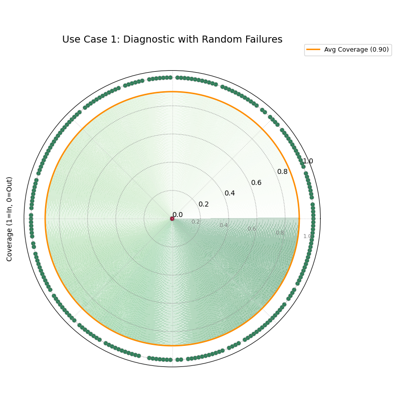
A diagnostic plot where successful coverages are green dots at radius 1, and failures are red dots at radius 0. The failures are scattered randomly.

🧠 Analysis and Interpretation

This plot provides a point-wise report card. The vast majority of points are green and lie on the outer circle at radius 1, indicating successful coverage. The few red points at radius 0 represent the interval failures. Critically, these red points are scattered randomly around the circle, with no obvious clusters or patterns. The solid orange line, representing the average coverage, sits at a radius of 0.90, confirming the model is well-calibrated. This random scatter of failures is the signature of a healthy, reliable model.

---

Use Case 2: Diagnosing Seasonal Model Failure

A model’s greatest weakness is often hidden in patterns. An aggregate coverage score might look good, but what if all the failures occur during a specific, critical season? This is a common and dangerous problem that this diagnostic plot is perfectly designed to uncover.

Let’s simulate a weather forecast model that is reliable most of the year but systematically fails during the summer heatwaves.

# --- 1. Data Generation: Seasonal Failures ---
np.random.seed(42)
n_days = 365
days_of_year = np.arange(n_days)
df_seasonal = pd.DataFrame({'day': days_of_year})
df_seasonal['actual_temp'] = 15 + 10 * np.sin(days_of_year * 2 * np.pi / 365) + np.random.normal(0, 2, n_days)
# Model produces intervals that are too narrow only during summer (days 150-240)
interval_width = np.ones(n_days) * 8
interval_width[(days_of_year > 150) & (days_of_year < 240)] = 3
df_seasonal['q10_temp'] = df_seasonal['actual_temp'] - interval_width
df_seasonal['q90_temp'] = df_seasonal['actual_temp'] + interval_width
# Manually push some summer actuals outside the narrow bounds
summer_indices = np.where((days_of_year > 150) & (days_of_year < 240))[0]
fail_indices = np.random.choice(summer_indices, 40, replace=False)
df_seasonal.loc[fail_indices, 'actual_temp'] += 5

# --- 2. Plotting with Bars for emphasis ---
kd.plot_coverage_diagnostic(
    df=df_seasonal,
    actual_col='actual_temp',
    q_cols=['q10_temp', 'q90_temp'],
    title='Use Case 2: Diagnosing Seasonal Failure',
    as_bars=True, # Use bars to highlight the cluster
    fill_gradient=False, # Turn off gradient to reduce clutter
    mask_angle=False, # Show the angular (day) labels
    verbose=0,
    savefig="gallery/images/gallery_coverage_diagnostic_seasonal.png"
)

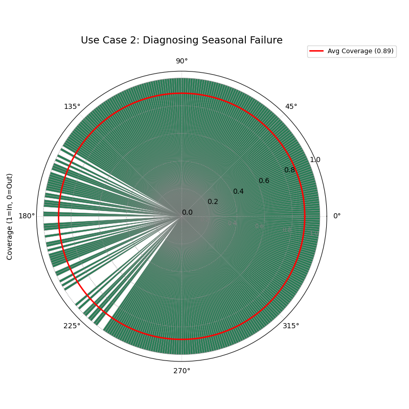
A diagnostic plot using bars, where a dense cluster of failures (bars at radius 0) is clearly visible in one sector of the plot.

🧠 Interpretation

This plot immediately reveals a critical, systematic failure in the model. While the overall coverage rate (solid red line) might still be reasonably high, there is a dense cluster of failures (bars at radius 0) concentrated in one specific angular sector. In this scenario, this corresponds to the summer months. This tells us the model’s uncertainty estimates are not robust; they are systematically too narrow and unreliable during summer, even though they perform well for the rest of the year. This is a clear signal that the model needs to be improved to handle seasonal volatility.

---

For a deeper understanding of the statistical concepts behind coverage and interval calibration, please refer back to the main Point-wise Coverage Diagnostic (plot_coverage_diagnostic()) section.

Interval Consistency

The plot_interval_consistency() function is an advanced diagnostic for assessing the stability of a model’s uncertainty estimates over time. While other plots show the magnitude of uncertainty at a single point, this visualization answers a deeper question: “Is my model’s assessment of its own uncertainty reliable and consistent from one forecast period to the next?”

Let’s begin by understanding the components of this powerful plot.

Plot Anatomy

• Angle (θ): Represents each individual sample or location, arranged sequentially around the circle by its DataFrame index. Since this ordering is often arbitrary, it is common to hide the angular tick labels using mask_angle=True.

• Radius (r): This is the key metric. It represents the variability of the interval width over multiple time steps for a single location. By default (use_cv=True), it is the Coefficient of Variation (CV), which measures relative variability. Points far from the center have highly inconsistent uncertainty estimates.

• Color: Provides context by representing the average median (Q50) prediction for each location across all time steps. This helps diagnose if inconsistency (high radius) is related to the magnitude of the prediction itself (color).

Now, let’s apply this diagnostic to a real-world problem, starting with a simple case and moving to a more complex one.

---

Use Case 1: Identifying Inconsistent Forecasts

The primary use of this plot is to identify locations where a model’s uncertainty estimates are unstable. A model that is very confident one year and very uncertain the next for the same location may not be trustworthy for long-term planning.

Let’s simulate multi-year river flow forecasts for a set of monitoring stations. Some stations will have stable uncertainty, while for others, it will fluctuate wildly.

import kdiagram as kd
import pandas as pd
import numpy as np
import matplotlib.pyplot as plt

# --- 1. Data Generation: Stable and Unstable Stations ---
np.random.seed(42)
n_stations = 150
years = [2021, 2022, 2023, 2024, 2025]
df = pd.DataFrame({'station_id': range(n_stations)})
qlow_cols, qup_cols, q50_cols = [], [], []

# Create a mix of stable and unstable stations
stable_mask = np.arange(n_stations) < 100
for year in years:
    # For unstable stations, width fluctuates randomly each year
    base_width = np.where(stable_mask, 10, 10 + np.random.uniform(-8, 8, n_stations))
    median = np.where(stable_mask, 50, 80) + np.random.randn(n_stations)*5
    df[f'q10_y{year}'] = median - base_width / 2
    df[f'q90_y{year}'] = median + base_width / 2
    df[f'q50_y{year}'] = median
    qlow_cols.append(f'q10_y{year}')
    qup_cols.append(f'q90_y{year}')
    q50_cols.append(f'q50_y{year}')

# --- 2. Plotting ---
kd.plot_interval_consistency(
    df=df,
    qlow_cols=qlow_cols,
    qup_cols=qup_cols,
    q50_cols=q50_cols,
    use_cv=True, # Radius = Coefficient of Variation
    title='Use Case 1: Identifying Unstable Uncertainty Forecasts',
    cmap='coolwarm',
    savefig="gallery/images/gallery_interval_consistency_basic.png"
)

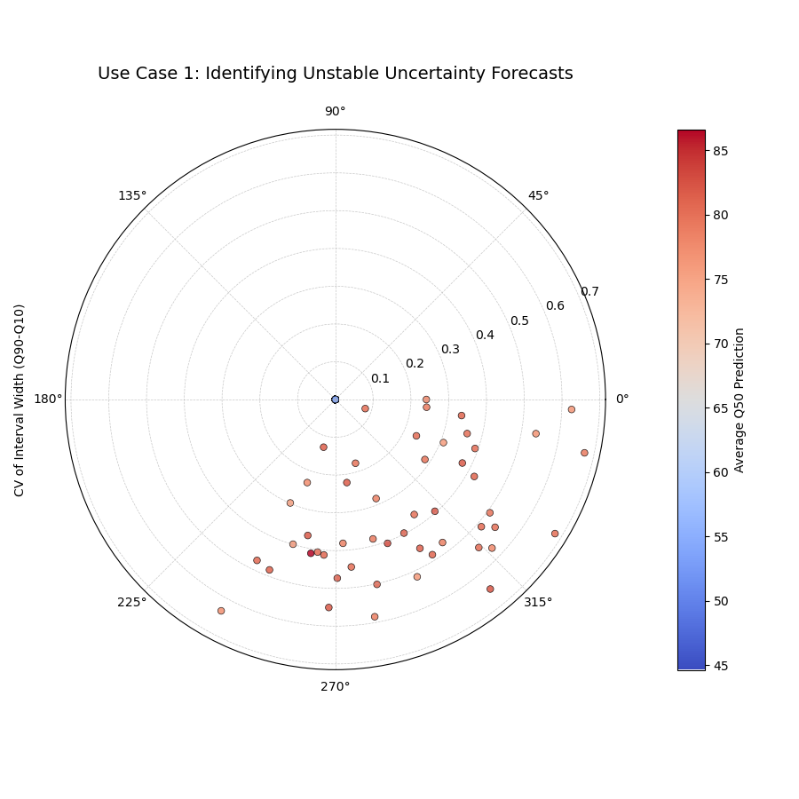
Most stations (points) are clustered near the center, indicating consistent uncertainty estimates, while a few outliers with large radii represent highly unstable forecasts.

🧠 Analysis and Interpretation

This plot effectively separates the forecasts with stable uncertainty from those with more volatile uncertainty. A significant cluster of points is visible very close to the center, indicating a low Coefficient of Variation (CV). For these stations, the model produces a stable and consistent prediction interval width year after year. The plot also reveals a second, more diffuse cloud of points at a larger radius, representing stations where the model’s assessment of its own uncertainty is moderately inconsistent. The color, representing the average predicted flow, appears reddish for most points, suggesting that both stable and unstable uncertainty estimates occur primarily for high-flow stations in this dataset.

---

Use Case 2: Comparing Absolute vs. Relative Variability

The choice between using the Coefficient of Variation (use_cv=True) and the Standard Deviation (use_cv=False) for the radius is an important one.

• CV measures relative inconsistency.

• Standard Deviation measures absolute inconsistency.

A station with a large average interval width might have a large standard deviation but a small CV, meaning it’s consistently uncertain. Let’s create a scenario to highlight this difference.

# --- 1. Data Generation: High vs. Low Flow Stations ---
np.random.seed(1)
n_stations = 100
years = [2021, 2022, 2023, 2024, 2025]
df_compare = pd.DataFrame({'id': range(n_stations)})
qlow_cols, qup_cols, q50_cols = [], [], []

# Low-flow stations: small but relatively inconsistent widths
low_flow_mask = np.arange(n_stations) < 50
for year in years:
    width = np.where(low_flow_mask, 2 + np.random.randn(n_stations), 20 + np.random.randn(n_stations))
    median = np.where(low_flow_mask, 10, 100)
    df_compare[f'q10_y{year}'] = median - width/2
    df_compare[f'q90_y{year}'] = median + width/2
    df_compare[f'q50_y{year}'] = median
    qlow_cols.append(f'q10_y{year}'); qup_cols.append(f'q90_y{year}'); q50_cols.append(f'q50_y{year}')

# --- 2. Create Side-by-Side Plots ---
fig, (ax1, ax2) = plt.subplots(1, 2, figsize=(16, 8), subplot_kw={'projection': 'polar'})

# Plot with Standard Deviation
kd.plot_interval_consistency(
    df=df_compare, ax=ax1, qlow_cols=qlow_cols, qup_cols=qup_cols, q50_cols=q50_cols,
    use_cv=False, title='Absolute Variability (Std. Dev.)', cmap='viridis'
)
# Plot with Coefficient of Variation
kd.plot_interval_consistency(
    df=df_compare, ax=ax2, qlow_cols=qlow_cols, qup_cols=qup_cols, q50_cols=q50_cols,
    use_cv=True, title='Relative Variability (CV)', cmap='viridis'
)

kd.savefig("gallery/images/gallery_interval_consistency_cv_vs_std.png")
plt.close(fig)

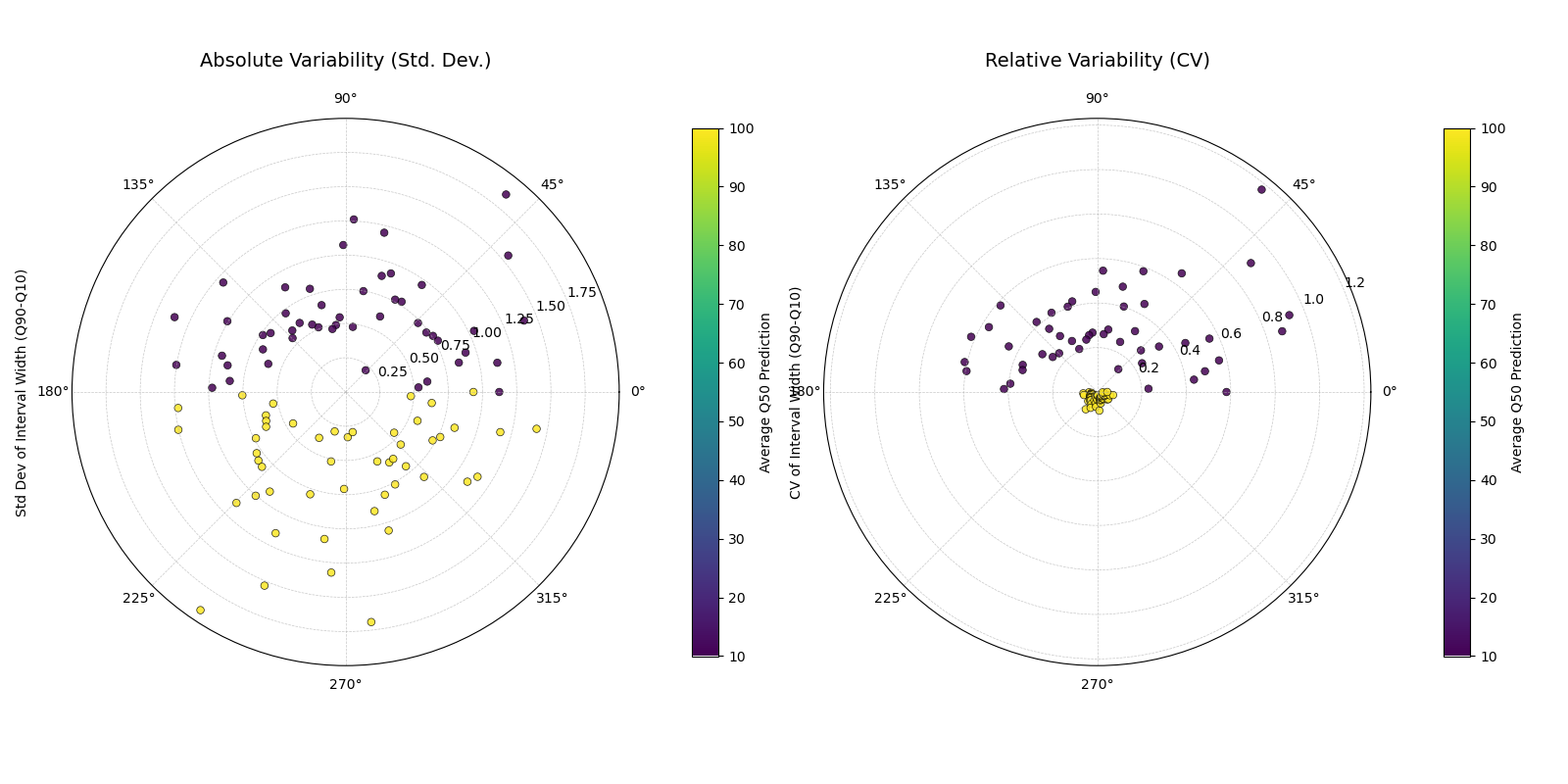
Two plots showing the same data. The left plot (Std. Dev.) shows the high-flow stations as more inconsistent. The right plot (CV) shows the low-flow stations are more inconsistent relative to their small average width.

🧠 Interpretation

This side-by-side comparison is extremely revealing. The left plot, using Standard Deviation, shows that the high-flow stations (yellow dots) have a much larger radius than the low-flow stations (purple dots). This tells us that in absolute terms, the interval width for high-flow stations fluctuates much more. However, the right plot, using the Coefficient of Variation, flips the story. Here, the low-flow stations (purple dots) are generally at a larger radius, meaning that relative to their small average width, their fluctuations are more significant and proportionally less predictable.

Best Practice

When comparing the stability of forecasts across different regimes (e.g., high-flow vs. low-flow stations), always check the consistency using both absolute (use_cv=False) and relative (use_cv=True) variability. The best choice depends on your application: if any absolute change is costly, use standard deviation. If you care more about proportional predictability, use CV.

---

For a deeper understanding of the statistical concepts behind forecast stability and variability, please refer back to the main Interval Width Consistency (plot_interval_consistency()) section.

Interval Width

The plot_interval_width() function is a specialized diagnostic tool for visualizing the magnitude of predicted uncertainty. It creates a polar scatter plot where the distance from the center (radius) directly represents the width of a model’s prediction interval for each sample. It is an essential tool for understanding a forecast’s sharpness and identifying patterns in its confidence.

Before exploring its applications, let’s first understand how to read this unique plot.

Plot Anatomy

• Angle (θ): Represents each individual sample’s position in the dataset, arranged sequentially around the circle by its DataFrame index. Since the index order is often arbitrary, the angular labels are typically hidden via mask_angle=True to avoid confusion.

• Radius (r): Directly corresponds to the prediction interval width (\(Q_{upper} - Q_{lower}\)). A larger radius means the model is predicting a wider range of outcomes and is therefore more uncertain for that specific sample.

• Color: Represents a third, contextual variable defined by the z_col parameter. This is usefull for diagnosing relationships, such as whether high uncertainty (large radius) correlates with high median predictions (e.g., bright colors).

With this framework, we can now apply the plot to a real-world problem, starting with a basic analysis and progressing to more advanced use cases.

---

Use Case 1: Basic Assessment of Uncertainty Spread

The most direct application of this plot is to get an immediate visual overview of the sharpness of a forecast. For a given set of predictions, are the uncertainty intervals generally wide or narrow? And is the uncertainty consistent across all samples?

Let’s simulate a forecast for a process where the uncertainty is expected to be relatively constant.

import kdiagram as kd
import pandas as pd
import numpy as np
import matplotlib.pyplot as plt

# --- 1. Data Generation: Constant Uncertainty ---
np.random.seed(10)
n_points = 200
df = pd.DataFrame({'sample_id': range(n_points)})
# A simple signal
df['q50_value'] = 50 + 10 * np.sin(np.linspace(0, 4 * np.pi, n_points))
# Constant interval width
width = np.random.normal(loc=15, scale=1.5, size=n_points)
df['q10_value'] = df['q50_value'] - width / 2
df['q90_value'] = df['q50_value'] + width / 2

# --- 2. Plotting ---
# We don't provide a z_col, so color will default to the radius (width)
kd.plot_interval_width(
    df=df,
    q_cols=['q10_value', 'q90_value'],
    title='Use Case 1: Basic Uncertainty Spread',
    cmap='cividis',
    cbar=True,
    s=35,
    savefig="gallery/images/gallery_interval_width_basic.png"
)
plt.close()

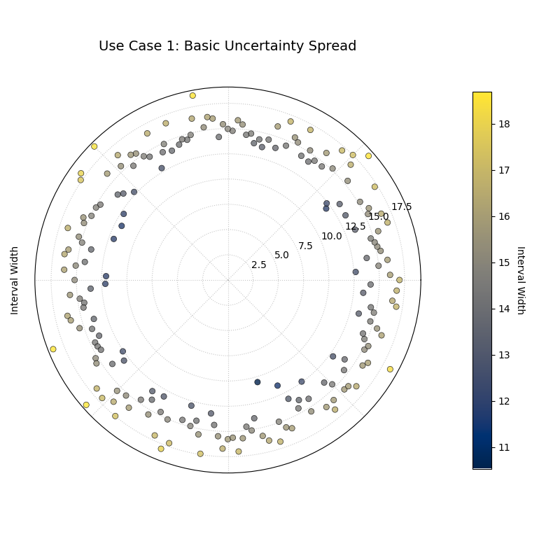
A ring of points where the radius (interval width) is fairly constant, indicating a homoscedastic forecast where uncertainty does not change across samples.

🧠 Analysis and Interpretation

This plot shows the interval width for 200 different samples. The key insight is that the points form a thin, circular ring at a nearly constant radius of approximately 15. This indicates that the model is homoscedastic—it predicts a consistent level of uncertainty for every sample in the dataset. The color, which in this case also represents the width, is uniform, reinforcing this finding. This is the expected behavior for many simple systems.

---

Use Case 2: Correlating Uncertainty with Forecast Magnitude

A more advanced use case is to investigate whether a model’s uncertainty is correlated with its own central prediction. A robust model should often be more uncertain when it is predicting extreme values. The z_col parameter is the key to unlocking this insight.

Let’s analyze a forecast for daily river flow, where we expect the uncertainty to be much higher during high-flow (flood) events.

# --- 1. Data Generation: Heteroscedastic Uncertainty ---
np.random.seed(77)
n_points = 200
df_river = pd.DataFrame({'day': range(n_points)})
# A signal representing seasonal river flow
df_river['q50_flow'] = 50 + 40 * np.sin(np.linspace(0, 2 * np.pi, n_points))**2
# Key: Interval width is now proportional to the median flow
width = 5 + (df_river['q50_flow'] * 0.3) * np.random.uniform(0.8, 1.2, n_points)
df_river['q10_flow'] = df_river['q50_flow'] - width
df_river['q90_flow'] = df_river['q50_flow'] + width

# --- 2. Plotting with z_col ---
kd.plot_interval_width(
    df=df_river,
    q_cols=['q10_flow', 'q90_flow'],
    z_col='q50_flow', # Color the points by the median prediction
    title='Use Case 2: River Flow Uncertainty (Colored by Median)',
    cmap='plasma',
    cbar=True,
    s=35,
    savefig="gallery/images/gallery_interval_width_correlated.png"
)
plt.close()

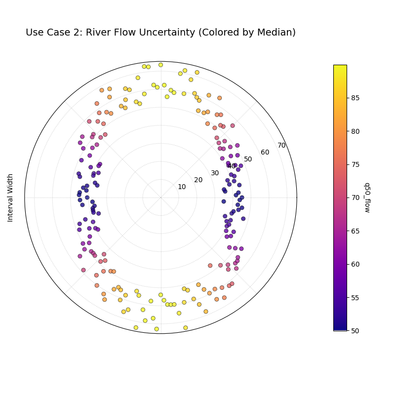
A spiral of points where both the radius (uncertainty) and the color (median flow) are low for some periods and high for others, showing a strong correlation.

🧠 Interpretation

This plot reveals a relationship in the forecast. The points form a spiral, not a simple ring. We can see that points with a small radius (low uncertainty) are dark purple, which the color bar tells us corresponds to a low median flow (q50_flow). Conversely, points with a large radius (high uncertainty) are bright yellow, corresponding to a high median flow. This is a clear visual confirmation of heteroscedasticity: the model has correctly learned to be more uncertain during high-flow periods and more confident during low-flow periods.

Best Practice

When diagnosing heteroscedasticity, setting z_col to your median prediction column (e.g., ‘q50’) is a good technique. A strong correlation between the radius (width) and the color (median) is often a sign of a well-behaved model that correctly scales its uncertainty with the magnitude of the phenomenon it is predicting.

---

For a deeper understanding of the statistical concepts behind forecast sharpness and heteroscedasticity, please refer back to the main Prediction Interval Width Visualization (plot_interval_width()) section.

Model Drift

The plot_model_drift() function is a specialized tool for diagnosing how a model’s performance degrades over longer prediction horizons. Using a polar bar chart, it visualizes how average uncertainty—or another metric of your choice—evolves as the forecast lead time increases, a phenomenon often called model drift.

First, let’s break down the components of this diagnostic chart.

Plot Anatomy

• Angle (θ): Each angular sector is assigned to a different forecast horizon (e.g., “1 Week Ahead”, “2 Weeks Ahead”). This creates a clear, sequential progression around the plot.

• Radius (r): Represents the average value of the primary metric for that horizon. By default, this is the mean prediction interval width (\(Q_{upper} - Q_{lower}\)), a measure of uncertainty. A longer bar means higher average uncertainty.

• Color: Provides a second dimension of information. By default, it also represents the primary metric (radius), but it can be mapped to a secondary metric (like average error) using the color_metric_cols parameter.

With this in mind, let’s apply the plot to a practical supply chain problem, starting with a basic uncertainty analysis and then adding a layer of complexity.

---

Use Case 1: Visualizing Uncertainty Drift

The most common use for this plot is to visualize how forecast sharpness degrades over time. A supply chain manager needs to understand how quickly the uncertainty in their demand forecast grows from one week to the next to manage inventory and mitigate the risk of stock-outs.

This example will show the average prediction interval width for demand forecasts at four different lead times.

import kdiagram as kd
import pandas as pd
import numpy as np
import matplotlib.pyplot as plt

# --- 1. Data Generation: Demand Forecasts for Multiple Horizons ---
np.random.seed(0)
n_samples = 100
horizons = ['1-Week Ahead', '2-Weeks', '3-Weeks', '4-Weeks']
df = pd.DataFrame()
q10_cols, q90_cols = [], []

for i, horizon in enumerate(horizons):
    # Uncertainty (interval width) increases with each horizon
    base_demand = 1000 + 50 * i
    interval_width = 100 + 50 * i
    q10 = base_demand - interval_width / 2 + np.random.randn(n_samples) * 20
    q90 = base_demand + interval_width / 2 + np.random.randn(n_samples) * 20
    df[f'q10_h{i+1}'] = q10
    df[f'q90_h{i+1}'] = q90
    q10_cols.append(f'q10_h{i+1}')
    q90_cols.append(f'q90_h{i+1}')

# --- 2. Plotting ---
kd.plot_model_drift(
    df=df,
    q10_cols=q10_cols,
    q90_cols=q90_cols,
    horizons=horizons,
    title='Use Case 1: Demand Forecast Uncertainty Drift',
    savefig="gallery/images/gallery_model_drift_basic.png"
)
plt.close()

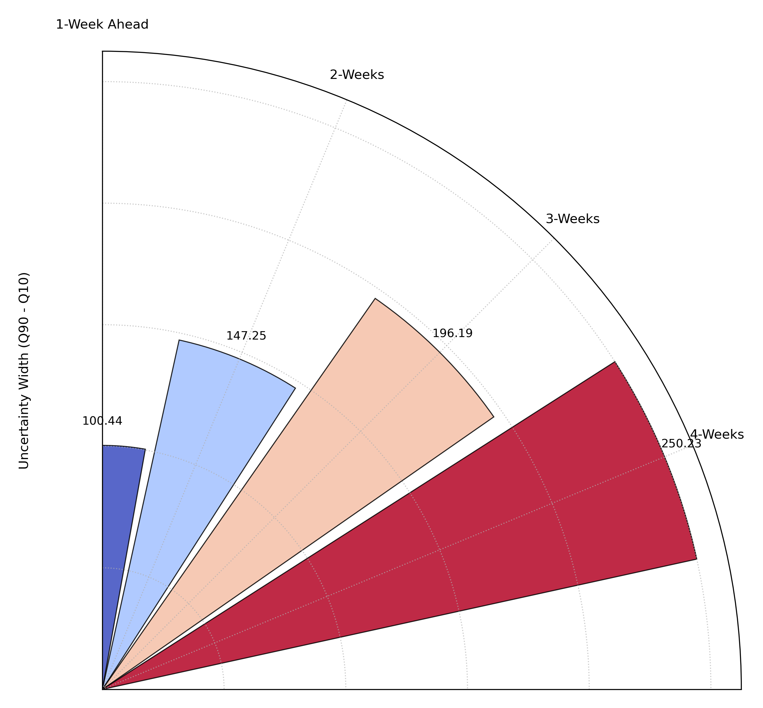
A polar bar chart where each bar represents a forecast horizon. The increasing height of the bars shows that the average prediction uncertainty grows as the forecast lead time increases.

🧠 Analysis and Interpretation

This plot provides a clear and intuitive summary of model drift. The height (radius) of each bar represents the average uncertainty for that forecast horizon. We can see a distinct and progressive increase in the bar heights as we move from the “1-Week Ahead” to the “4-Weeks Ahead” forecast. The annotations quantify this, showing the average interval width growing from ~100 (100.44) to over 250 units (250.23). This is a classic demonstration of model drift, where the forecast becomes rapidly less precise at longer lead times, a critical insight for inventory planning.

---

Use Case 2: Adding a Second Metric with Color

While uncertainty is critical, it’s only half the story. We also care about accuracy. Does the model’s error (e.g., Mean Absolute Error) also increase at longer horizons? The color_metric_cols parameter allows us to layer this second dimension of information onto our plot.

Let’s simulate the MAE for each horizon and use it to color the bars, giving us a simultaneous view of both uncertainty and accuracy drift.

# --- 1. Data Generation (assumes df from previous step is available) ---
# Simulate Mean Absolute Error (MAE) for each horizon, which also increases
mae_cols = []
for i, horizon in enumerate(horizons):
    # MAE increases with each horizon
    mae = 25 + 15 * i + np.random.uniform(-5, 5, n_samples)
    df[f'mae_h{i+1}'] = mae
    mae_cols.append(f'mae_h{i+1}')

# --- 2. Plotting with a secondary color metric ---
kd.plot_model_drift(
    df=df,
    q10_cols=q10_cols,
    q90_cols=q90_cols,
    horizons=horizons,
    color_metric_cols=mae_cols, # Use MAE to color the bars
    value_label="Avg. Uncertainty Width", # Label for radius
    # The color bar label is automatically inferred from the column names
    title='Use Case 2: Uncertainty Drift (Colored by MAE)',
    acov='eighth_circle',
    cmap='YlOrRd', # Use a sequential colormap for error
)
kd.savefig("gallery/images/gallery_model_drift_color.png")

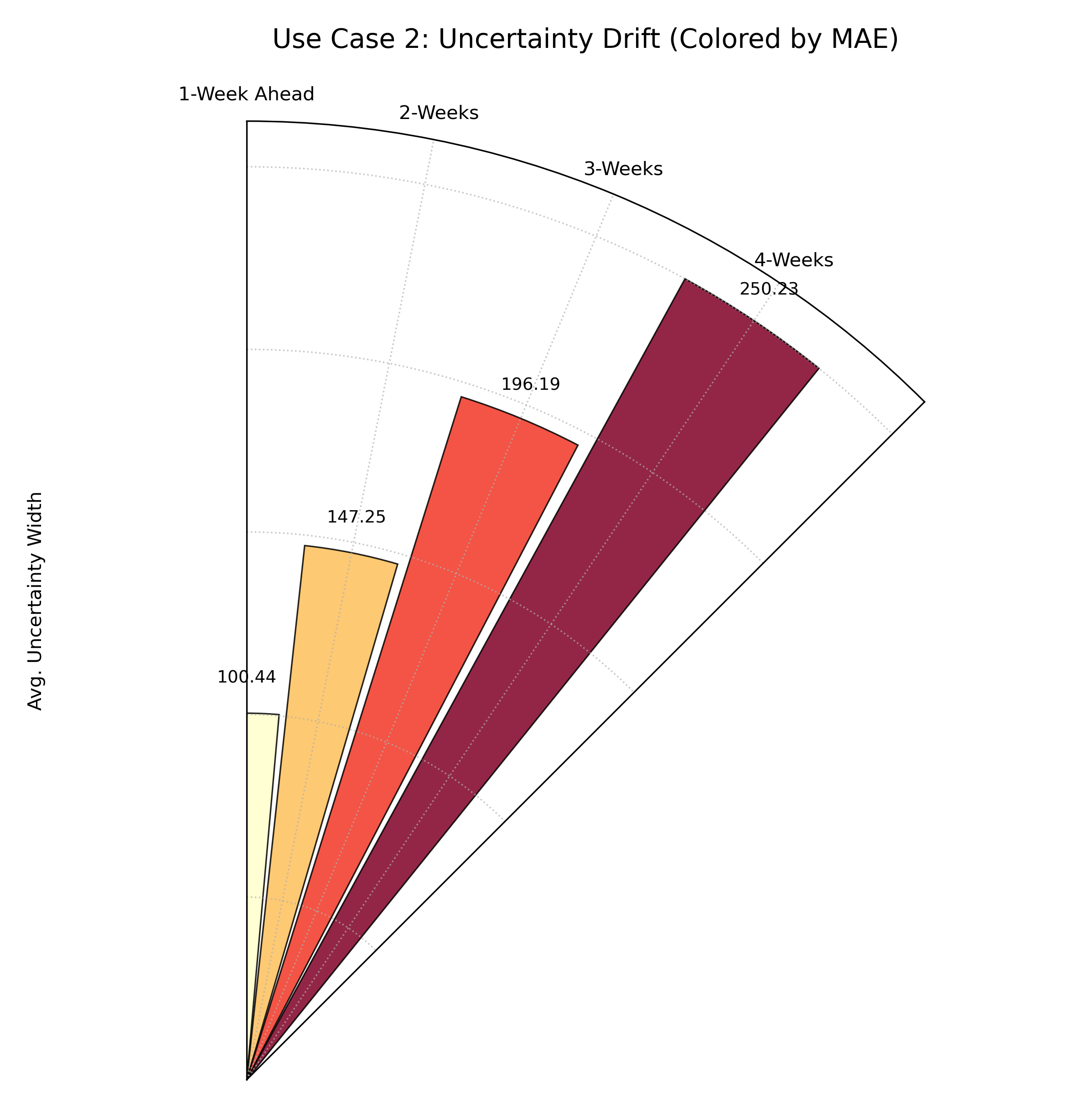
A polar bar chart where bar height still shows uncertainty, but the color now represents the average forecast error (MAE), with darker red indicating higher error.

🧠 Interpretation

This enhanced plot now tells a richer story. As before, the increasing height of the bars shows that the forecast uncertainty is growing. In addition, the color of the bars—which now represents the average MAE—is getting progressively darker and redder. This confirms our hypothesis: as the forecast horizon extends, the model becomes not only less certain (wider intervals) but also less accurate (higher error). This two-dimensional diagnostic provides a more complete picture of performance degradation.

---

For a deeper understanding of the statistical concepts behind model drift and forecast evaluation, please refer back to the main Evaluating Classification Models and Model Forecast Drift (plot_model_drift()) sections.

Temporal Uncertainty

The plot_temporal_uncertainty() function is a flexible, general-purpose tool for visualizing and comparing multiple data series in a polar context. While it can be used for many tasks, its primary application is to display the full spread of a probabilistic forecast at a single point in time by plotting several of its predicted quantiles simultaneously.

Let’s first break down the components of this versatile plot.

Plot Anatomy

• Angle (θ): Represents each individual sample’s position in the dataset, arranged sequentially around the circle by its DataFrame index. As this index order may not always be meaningful, it is often best practice to hide the angular labels by setting mask_angle=True.

• Radius (r): Corresponds to the magnitude of the predicted value for each specific quantile series. When normalize=False, this shows the raw predicted values (e.g., stock price). When normalize=True, it shows the relative position of the prediction within that series’ own min-max range.

• Color: Each data series (e.g., Q10, Q25, Q50) is assigned a distinct color from the chosen cmap, making it easy to distinguish the different layers of the forecast.

With this in mind, let’s explore how this plot can be used to analyze a complex financial forecast.

---

Use Case 1: Visualizing a Symmetric Forecast Distribution

The most common use case is to visualize the shape and spread of a forecast’s uncertainty. A well-behaved, simple forecast might produce a symmetrical uncertainty distribution around its median prediction.

Let’s simulate a forecast for a stock’s price over 100 days, where the predicted uncertainty is stable and symmetric.

import kdiagram as kd
import pandas as pd
import numpy as np
import matplotlib.pyplot as plt

# --- 1. Data Generation: Symmetric Uncertainty ---
np.random.seed(42)
n_days = 100
base_price = 150 + np.cumsum(np.random.randn(n_days))
df = pd.DataFrame()
# Symmetrical quantiles around a median (Q50)
df['q10'] = base_price - 15
df['q25'] = base_price - 7
df['q50'] = base_price
df['q75'] = base_price + 7
df['q90'] = base_price + 15

# --- 2. Plotting ---
kd.plot_temporal_uncertainty(
    df=df,
    q_cols=['q10', 'q25', 'q50', 'q75', 'q90'],
    names=['Q10', 'Q25', 'Median', 'Q75', 'Q90'],
    normalize=False, # Plot actual price values
    title='Use Case 1: Symmetric Stock Price Forecast',
    savefig="gallery/images/gallery_temporal_uncertainty_symmetric.png"
)

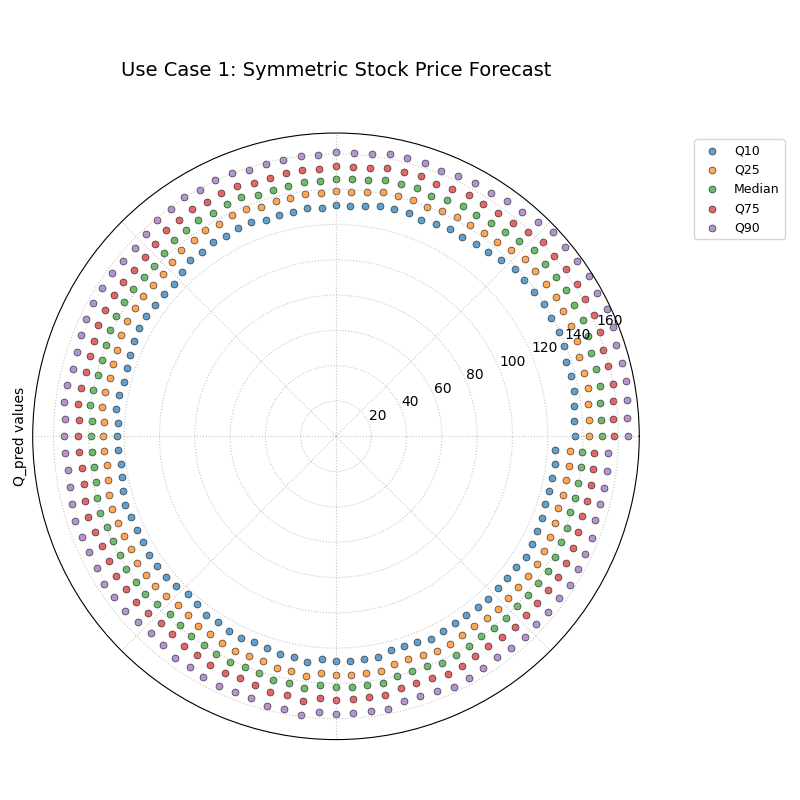
Five concentric, parallel rings of points, representing a symmetric probabilistic forecast where the uncertainty spread is constant.

🧠 Analysis and Interpretation

This plot visualizes the entire forecast distribution for each day. We see five distinct, roughly parallel spirals, each representing a quantile. The radial distance between the outermost (Q90) and innermost (Q10) spirals represents the width of the 80% prediction interval. The key insight here is that the spacing between the quantile spirals is symmetrical and constant. The distance from Q10 to Q25 is the same as from Q75 to Q90, and the Q50 (median) is perfectly centered. This is the signature of a simple, symmetric uncertainty forecast.

---

Use Case 2: Diagnosing Skewed Uncertainty

Real-world uncertainty is often not symmetric. For example, a stock’s price might have a much larger potential upside (risk of a price surge) than a downside. This plot is an ideal tool for diagnosing such skewed distributions.

Let’s simulate a forecast for a volatile tech stock, where the model predicts a greater chance of large positive returns than large negative ones.

# --- 1. Data Generation: Skewed Uncertainty ---
np.random.seed(10)
n_days = 100
base_price = 150 + np.cumsum(np.random.randn(n_days))
df_skewed = pd.DataFrame()
# Asymmetrical quantiles: larger gap on the upside
df_skewed['q10'] = base_price - 5
df_skewed['q25'] = base_price - 2
df_skewed['q50'] = base_price
df_skewed['q75'] = base_price + 8  # Larger step
df_skewed['q90'] = base_price + 20 # Much larger step

# --- 2. Plotting ---
kd.plot_temporal_uncertainty(
    df=df_skewed,
    q_cols=['q10', 'q25', 'q50', 'q75', 'q90'],
    normalize=False,
    title='Use Case 2: Skewed Stock Price Forecast',
    savefig="gallery/images/gallery_temporal_uncertainty_skewed.png"
)

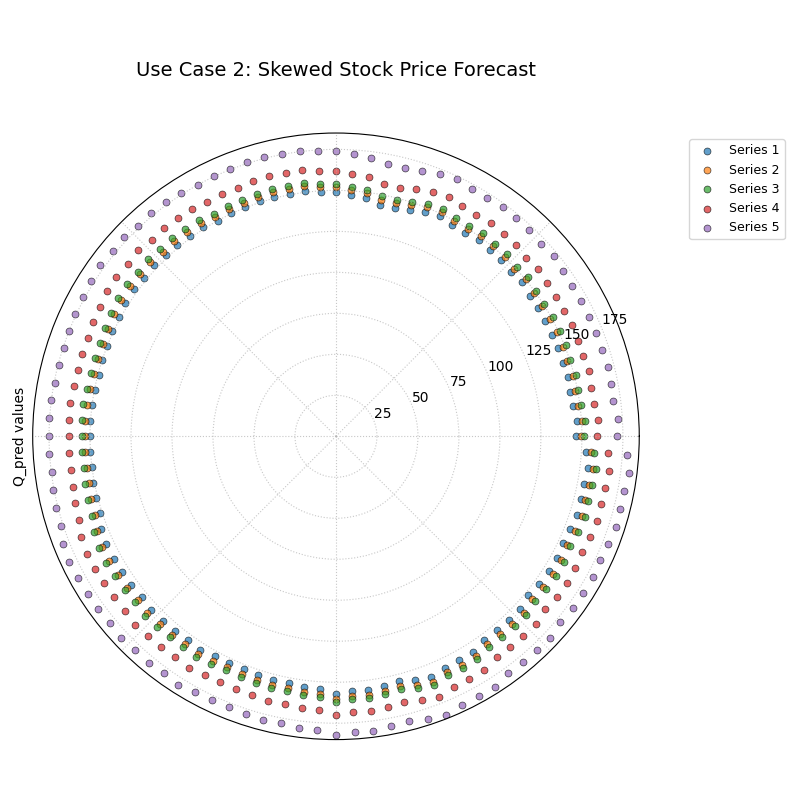
Five concentric rings of points that are not evenly spaced. The outer rings (Q75, Q90) are much further apart than the inner rings (Q10, Q25).

🧠 Interpretation

Unlike the first example, the spacing between the quantile spirals is now clearly asymmetrical. The radial distance between the upper quantiles (Q75 and Q90) is much larger than the distance between the lower quantiles (Q10 and Q25). This plot immediately reveals that the model is predicting a positively skewed distribution. It forecasts a limited downside risk but a much larger potential for significant positive price movements, an important insight for any trading or investment strategy.

---

For a deeper understanding of the statistical concepts behind probabilistic forecasting and quantile analysis, please refer back to the main General Polar Series Visualization (plot_temporal_uncertainty()) section.

Uncertainty Drift

The plot_uncertainty_drift() function is a tool for visualizing how an entire spatial pattern of uncertainty evolves over multiple time steps. Unlike plots that show an average drift, this visualization uses concentric rings to display a complete “map” of uncertainty for each forecast period, allowing you to diagnose complex spatiotemporal changes.

Let’s begin by understanding the components of this innovative plot.

Plot Anatomy

• Angle (θ): Represents each individual sample or location in the dataset, arranged sequentially around the circle. For geospatial data, this could correspond to longitude or a station index. Since the raw index may not be meaningful, it’s common to hide the angular tick labels with mask_angle=True.

• Concentric Rings: Each colored ring corresponds to a different time step or forecast horizon (e.g., Year 1, Year 2). Later time steps are plotted on outer rings.

• Radius (r) of a Ring: The radius of the line on any given ring is a combination of a base offset (to separate the rings) and a component proportional to the globally normalized interval width. Therefore, “bumps” or outward bulges in a ring signify regions of higher relative uncertainty at that time step.

Now, let’s apply this plot to a critical environmental forecasting problem.

---

Use Case 1: Identifying Uniform Uncertainty Growth

In the simplest scenario, a model’s uncertainty might be expected to grow uniformly over time and across all locations. This plot can validate that assumption.

Let’s simulate a multi-year land subsidence forecast for a region where we expect the uncertainty to increase at the same rate everywhere.

import kdiagram as kd
import pandas as pd
import numpy as np
import matplotlib.pyplot as plt

# --- 1. Data Generation: Uniform Drift ---
np.random.seed(55)
n_locations = 100
years = [2024, 2025, 2026, 2027]
df = pd.DataFrame({'id': range(n_locations)})
qlow_cols, qup_cols = [], []

for i, year in enumerate(years):
    ql, qu = f'subsidence_{year}_q10', f'subsidence_{year}_q90'
    qlow_cols.append(ql); qup_cols.append(qu)
    # Uncertainty width increases with the year, but is uniform across locations
    width = 2.0 + i * 1.5
    median = 10 + i * 2
    df[ql] = median - width / 2
    df[qu] = median + width / 2

# --- 2. Plotting ---
kd.plot_uncertainty_drift(
    df=df,
    qlow_cols=qlow_cols,
    qup_cols=qup_cols,
    dt_labels=[str(y) for y in years],
    title='Use Case 1: Uniform Uncertainty Drift',
    savefig="gallery/images/gallery_uncertainty_drift_uniform.png"
)

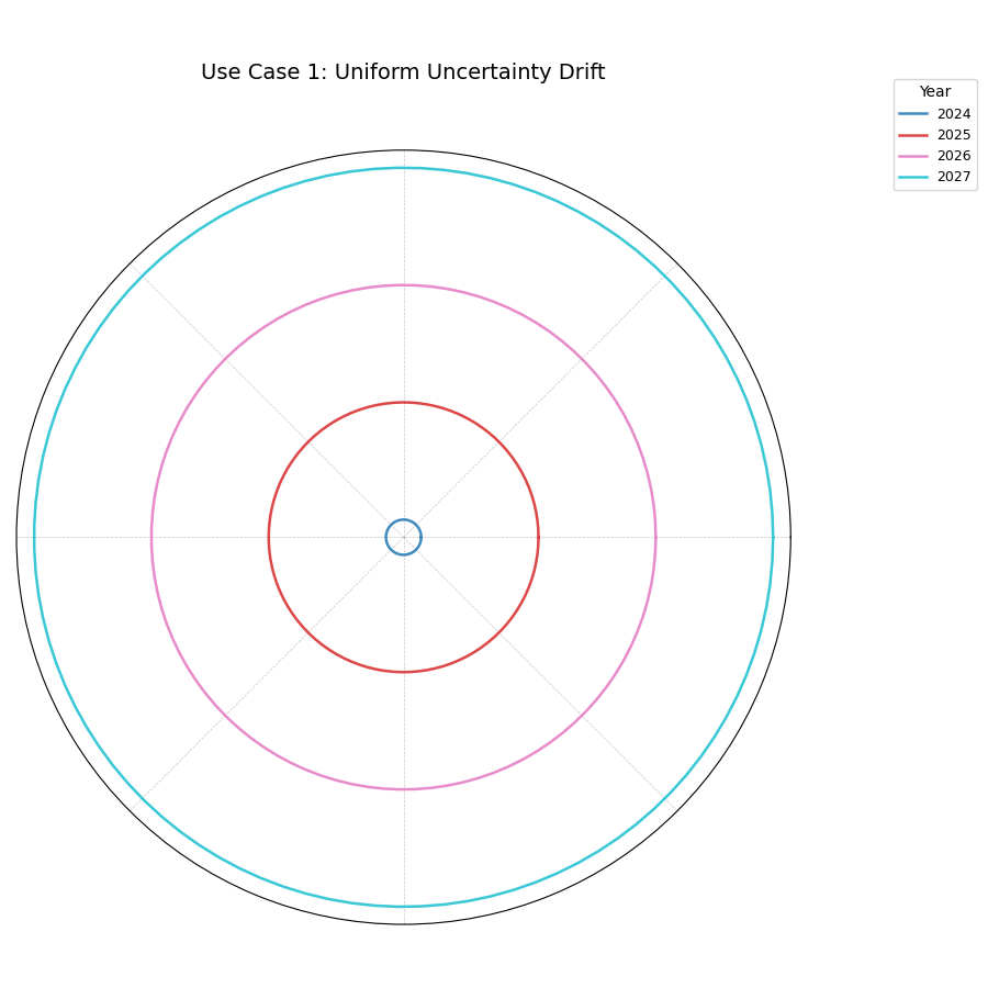
A series of perfectly circular and evenly spaced concentric rings, each representing a year. This indicates that uncertainty grows uniformly over time and space.

🧠 Analysis and Interpretation

This plot shows four perfectly circular rings, one for each year. The key insights are twofold. First, the radius of the rings steadily increases from 2024 (innermost) to 2027 (outermost), confirming that the average forecast uncertainty is growing over time. Second, each ring is a perfect circle, which means that for any given year, the predicted uncertainty is the same for all locations. This is the signature of a simple, uniform uncertainty drift.

---

Use Case 2: Diagnosing Spatiotemporal Drift

More realistically, a model’s uncertainty drift is not uniform. Certain regions may become unpredictable much faster than others. This plot excels at revealing these complex, combined spatial and temporal patterns.

Let’s simulate a more realistic scenario where subsidence uncertainty grows much faster in a specific, localized region.

# --- 1. Data Generation: Spatiotemporal Drift ---
np.random.seed(1)
n_locations = 200
locations_angle = np.linspace(0, 360, n_locations, endpoint=False)
df_spatial = pd.DataFrame({'id': range(n_locations)})
years = [2024, 2025, 2026, 2027]
qlow_cols, qup_cols = [], []

for i, year in enumerate(years):
    ql, qu = f'subsidence_{year}_q10', f'subsidence_{year}_q90'
    qlow_cols.append(ql); qup_cols.append(qu)
    # Uncertainty grows over time AND in a specific region (90-180 degrees)
    regional_effect = (locations_angle > 90) & (locations_angle < 180)
    base_width = 5 + 2 * i
    width = base_width + np.where(regional_effect, 8 * i, 0) # Strong regional growth
    median = 10
    df_spatial[ql] = median - width / 2
    df_spatial[qu] = median + width / 2

# --- 2. Plotting ---
kd.plot_uncertainty_drift(
    df=df_spatial,
    qlow_cols=qlow_cols,
    qup_cols=qup_cols,
    dt_labels=[str(y) for y in years],
    title='Use Case 2: Diagnosing Spatiotemporal Drift',
    cmap='plasma',
    savefig="gallery/images/gallery_uncertainty_drift_spatial.png"
)

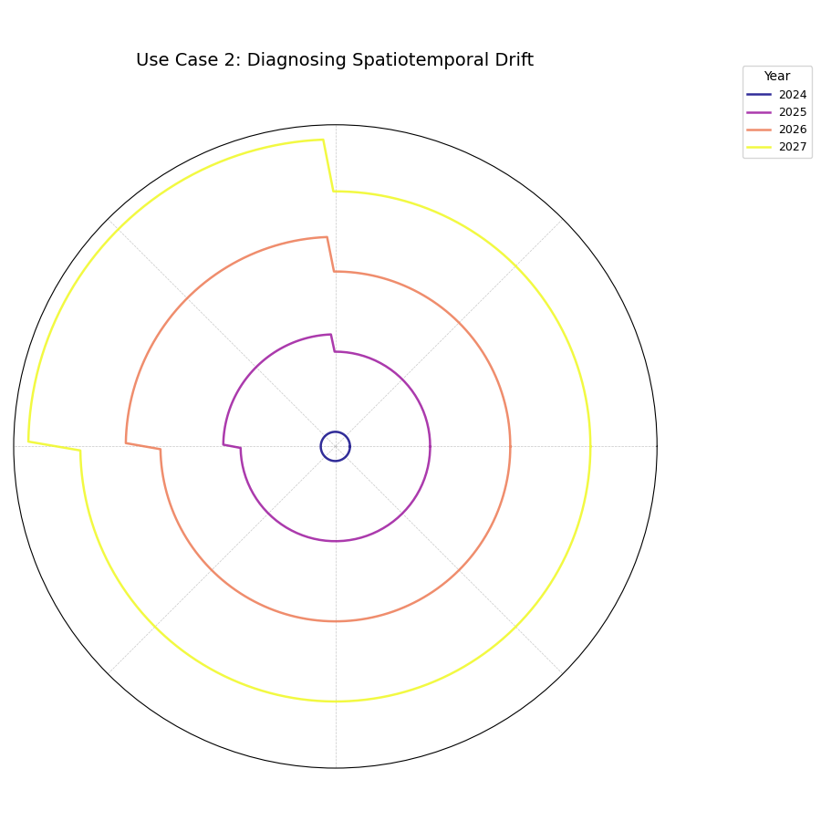
A series of concentric rings where a distinct “bulge” or outward protrusion appears in the top-left quadrant and grows larger with each successive year.

🧠 Interpretation

This plot immediately reveals a complex spatiotemporal pattern. While all the rings grow larger from 2024 to 2027, indicating a general increase in uncertainty over time, they are no longer perfect circles. A significant “bulge” has developed in the top-left quadrant (from 90° to 180°). This bulge becomes progressively more pronounced in the outer rings (later years). This is a perfect insight: it tells us that not only is uncertainty growing, but it is growing much faster in this specific geographic region, which should be the highest priority for monitoring.

See Also

The plot_model_drift() function provides a complementary view. While this plot shows the full spatial pattern of uncertainty drift, plot_model_drift focuses on the average drift across all locations, summarizing it with a simple bar chart. Using both provides a complete picture.

---

For a deeper understanding of the statistical concepts behind spatiotemporal uncertainty and model drift, please refer back to the main Multi-Time Uncertainty Drift Rings (plot_uncertainty_drift()) section.

Prediction Velocity

The plot_velocity() function moves beyond static predictions to visualize the dynamics of change. It calculates the average rate of change (or “velocity”) of a forecast’s central tendency over time for multiple locations. This is essential for identifying “hotspots” where a phenomenon is changing most rapidly and for understanding the underlying trends in a system.

First, let’s explore the components of this dynamic visualization.

Plot Anatomy

• Angle (θ): Represents each individual sample or location, arranged sequentially around the circle by its DataFrame index. Since this ordering is often arbitrary, the angular labels can be hidden with mask_angle=True to focus on the radial patterns.

• Radius (r): Corresponds to the average velocity of the median (Q50) prediction over the specified time steps. A larger radius signifies a faster average rate of change for that location. The radius can be normalized or shown in its raw units.

• Color: Provides a crucial second layer of context. It can either represent the average absolute magnitude of the prediction (use_abs_color=True) or the velocity itself (use_abs_color=False), which is usefull for showing the direction of change.

With this framework, let’s apply the plot to a critical environmental monitoring problem.

---

Use Case 1: Identifying Hotspots of Change

The most direct use of this plot is to identify which locations are changing the fastest. We can visualize the rate of change (velocity) as the radius and use color to provide context about the absolute state of each location.

Let’s simulate a multi-year forecast of land subsidence (sinking) for various locations in a coastal city. The primary goal is to find the areas that are sinking most rapidly.

import kdiagram as kd
import pandas as pd
import numpy as np
import matplotlib.pyplot as plt

# --- 1. Data Generation: Land Subsidence Forecast ---
np.random.seed(42)
n_locations = 150
df = pd.DataFrame({'location_id': range(n_locations)})
years = [2024, 2025, 2026, 2027]
q50_cols = []
# Assign a base subsidence level and a variable velocity to each location
base_subsidence = np.random.uniform(5, 20, n_locations)
velocity = np.linspace(0.5, 5, n_locations) # Some sink slow, some fast
np.random.shuffle(velocity) # Randomize the velocities

for i, year in enumerate(years):
    q50_col = f'subsidence_{year}_q50'
    q50_cols.append(q50_col)
    df[q50_col] = base_subsidence + velocity * i

# --- 2. Plotting ---
kd.plot_velocity(
    df=df,
    q50_cols=q50_cols,
    title='Use Case 1: Land Subsidence Velocity Hotspots',
    use_abs_color=True, # Color by total subsidence magnitude
    normalize=True,     # Normalize velocity for a clear [0,1] radius
    cmap='plasma',
    cbar=True,
    s=35,
    savefig="gallery/images/gallery_velocity_basic.png"
)

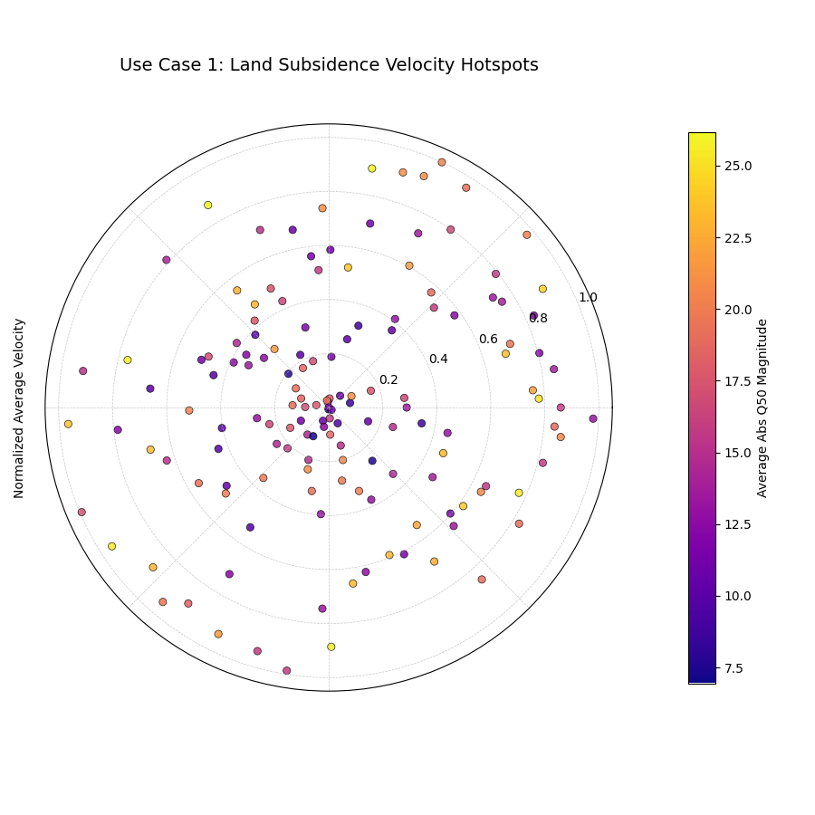
Points spiraling outwards, where the distance from the center (radius) indicates the normalized rate of sinking, and the color indicates the average total subsidence.

🧠 Analysis and Interpretation

This plot effectively identifies hotspots of change. The radius of each point represents its normalized velocity, so points at the outer edge of the spiral are the locations predicted to sink the fastest. The color, representing the average total subsidence, adds critical context. The spiral transitions from dark purple (low total subsidence) to bright yellow (high total subsidence). The key insight is the strong correlation: the locations sinking the fastest (large radius) are also the ones with the highest overall subsidence (bright yellow). This tells planners that the most critical areas are continuing to degrade at the highest rates.

---

Use Case 2: Distinguishing Direction of Change

Beyond just the speed of change, we often need to know the direction. Is a value increasing or decreasing? By setting use_abs_color=False and using a diverging colormap, we can use color to represent the direction and magnitude of the velocity itself.

Let’s analyze a forecast of glacier mass balance (the net gain or loss of ice) for different glaciers. Some are predicted to grow (positive velocity), while most are predicted to shrink (negative velocity).

# --- 1. Data Generation: Glacier Mass Balance ---
np.random.seed(1)
n_glaciers = 100
df_glaciers = pd.DataFrame({'glacier_id': range(n_glaciers)})
years = [2025, 2030, 2035, 2040]
q50_cols = []
# Most glaciers are shrinking (negative velocity)
base_mass = np.random.uniform(100, 500, n_glaciers)
velocity = np.random.normal(-10, 3, n_glaciers)
# A few are stable or growing
velocity[np.random.choice(n_glaciers, 10, replace=False)] *= -0.5

for i, year in enumerate(years):
    q50_col = f'mass_{year}_q50'
    q50_cols.append(q50_col)
    df_glaciers[q50_col] = base_mass + velocity * i

# --- 2. Plotting with color representing velocity direction ---
kd.plot_velocity(
    df=df_glaciers,
    q50_cols=q50_cols,
    title='Use Case 2: Glacier Mass Balance Velocity',
    use_abs_color=False, # Color by velocity itself
    normalize=False,     # Use raw velocity for the radius
    cmap='coolwarm',     # A diverging colormap (blue-white-red)
    cbar=True,
    savefig="gallery/images/gallery_velocity_directional.png"
)

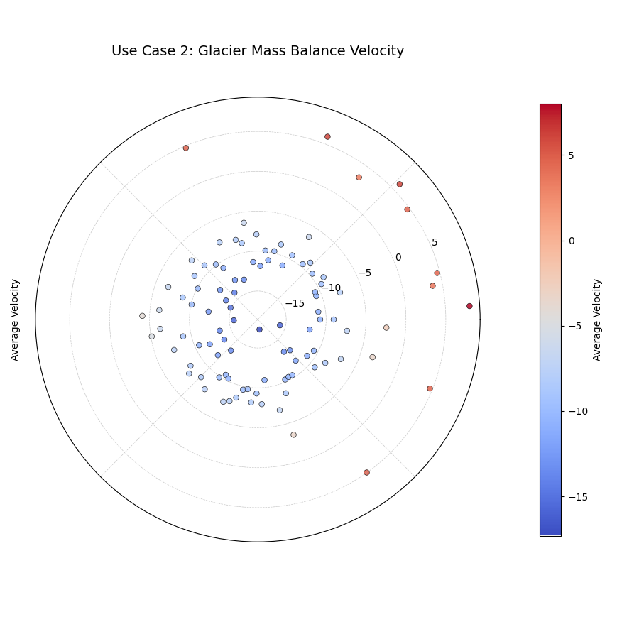
Points colored with a diverging colormap. The blue points show a negative velocity (shrinking), while the few red points show a positive velocity (growing).

🧠 Interpretation

This plot now clearly distinguishes the direction of change. By using a diverging colormap like coolwarm, the color directly tells us the sign of the velocity. The vast majority of points are blue, indicating a negative velocity—these are the glaciers predicted to lose mass (<0). The few red points represent the rare glaciers predicted to grow (>=0). The radius still represents the magnitude of this change, so the blue points furthest from the center are the glaciers predicted to be shrinking the fastest.

Best Practice

When your data’s rate of change can be both positive and negative, set use_abs_color=False and choose a diverging cmap (like coolwarm, RdBu, or seismic). This is the most effective way to visually separate trends of increase versus decrease.

---

For a deeper understanding of the statistical concepts behind analyzing temporal trends, please refer back to the main Prediction Velocity Visualization (plot_velocity()) section.

Radial Density Ring

The plot_radial_density_ring() function offers a unique and interesting way to visualize the shape of a one-dimensional probability distribution. It transforms a standard histogram or density plot into a smooth, continuous polar ring, where the color intensity reveals the most common values. This is an invaluable tool for understanding the fundamental character of your data, be it forecast errors, interval widths, or any other continuous metric.

Let’s begin by understanding the components of this elegant visualization.

Plot Anatomy

• Angle (θ): The angular dimension carries no information in this plot. The density is repeated around the full circle purely for aesthetic effect, creating the “ring” shape. The angular labels are therefore hidden by default.

• Radius (r): Directly corresponds to the value of the variable being analyzed (e.g., forecast error, interval width). The radial axis represents the domain of your data.

• Color: Represents the normalized probability density at each radial position, calculated via Kernel Density Estimation (KDE). Bright, intense colors indicate the most common values (the peaks, or modes, of the distribution).

This function can derive the data to be plotted in three different ways using the kind parameter. Let’s explore each one with a practical example.

---

Use Case 1: Distribution of a Direct Metric (``kind=’direct’``)

The most straightforward use of this plot is to visualize the distribution of any single, pre-existing column in your data. A classic application is to examine the distribution of model errors (residuals) to check for bias.

An unbiased model should have errors centered symmetrically around zero. Let’s check if our simulated model meets this crucial criterion.

import kdiagram as kd
import pandas as pd
import numpy as np
import matplotlib.pyplot as plt

# --- 1. Data Generation (shared for all examples) ---
np.random.seed(42)
n_samples = 1000
df_test = pd.DataFrame({
    'q10': np.random.normal(10, 2, n_samples),
    'q90': np.random.normal(30, 3, n_samples),
    'value_2022': np.random.gamma(3, 5, n_samples),
    'value_2023': np.random.gamma(4, 5, n_samples),
    'error_metric': np.random.normal(loc=2.5, scale=5, size=n_samples) # A biased error
})
# Ensure q90 is always greater than q10
df_test['q90'] = df_test[['q10', 'q90']].max(axis=1) + np.random.rand(n_samples) * 2

# --- 2. Plotting ---
kd.plot_radial_density_ring(
    df=df_test,
    kind="direct",
    target_cols="error_metric",
    title="Use Case 1: Distribution of Model Errors",
    cmap="viridis",
    r_label="Forecast Error",
    savefig="gallery/images/gallery_plot_density_ring_direct.png"
)

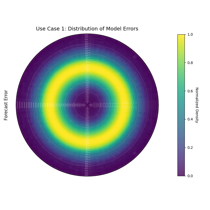
A density ring where the brightest color is not at the center (radius 0), indicating a biased error distribution.

🧠 Analysis and Interpretation

This plot visualizes the distribution of our model’s errors. For an unbiased model, the brightest part of the ring should be centered perfectly at a radius of 0. Here, however, the bright yellow ring is clearly centered at a positive radius of approximately +2.5. This instantly reveals a systemic positive bias in the forecast; the model, on average, under-predicts the true value by 2.5 units. The symmetric, bell-like shape of the ring suggests the errors are otherwise normally distributed, but their center is in the wrong place.

---

Use Case 2: Distribution of Interval Width (``kind=’width’``)

A crucial aspect of a probabilistic forecast is its sharpness, which is measured by the prediction interval width. This plot can help us understand the characteristics of our model’s uncertainty estimates. Are they consistent, or do they vary wildly?

Let’s visualize the distribution of the interval width calculated from our simulated forecast’s 10th and 90th percentiles.

# --- 1. Data Generation (uses df_test from previous step) ---

# --- 2. Plotting ---
kd.plot_radial_density_ring(
    df=df_test,
    kind="width",
    target_cols=["q10", "q90"],
    title="Use Case 2: Distribution of Interval Width",
    cmap="magma",
    r_label="Interval Width (q90 - q10)",
    savefig="gallery/images/gallery_plot_density_ring_width.png"
)

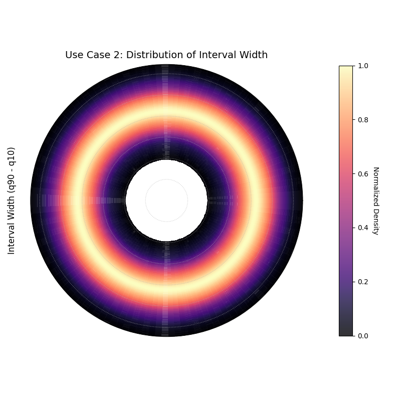
A density ring showing that the most common interval width is approximately 22 units.

🧠 Interpretation

This plot reveals the distribution of the model’s predicted uncertainty. The brightest part of the ring is centered around a radius of approximately 22. This tells us that the most common prediction interval width produced by the model is 22 units. The distribution is fairly symmetric and tight, suggesting the model produces a relatively consistent level of uncertainty for most samples. A very wide or multi-peaked ring would indicate more erratic uncertainty estimation.

---

Use Case 3: Distribution of Change (``kind=’velocity’``)

This mode is perfect for analyzing the distribution of change between two time points or a “velocity.” This is invaluable for understanding the dynamics of a system. Is change typically small and centered around zero, or are large shifts common?

Let’s analyze the year-over-year change in our simulated gamma-distributed values from 2022 to 2023.

# --- 1. Data Generation (uses df_test from previous step) ---

# --- 2. Plotting ---
kd.plot_radial_density_ring(
    df=df_test,
    kind="velocity",
    target_cols=["value_2022", "value_2023"],
    title="Use Case 3: Distribution of Year-over-Year Change",
    cmap="inferno",
    r_label="Change (value_2023 - value_2022)",
    savefig="gallery/images/gallery_plot_density_ring_velocity.png"
)

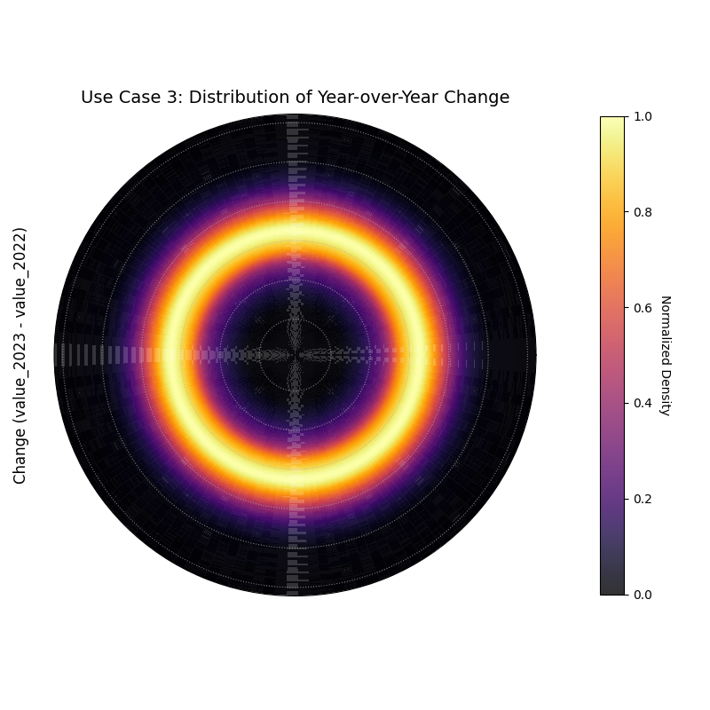
A density ring showing that the most common year-over-year change was a positive increase of about 5 units.

🧠 Interpretation

This plot shows the distribution of the year-over-year change in our variable. The brightest part of the ring is centered at a positive radius of about +5. This indicates that the most common change from 2022 to 2023 was an increase of 5 units. The distribution is also positively skewed, with a “tail” of brighter color extending to larger positive radii. This suggests that while a +5 change was most typical, some samples experienced a much larger positive increase, while large decreases were rare.

---

Use Case 4: Comparing Conditional Distributions

A truly usefull application of this plot is to move beyond analyzing a single dataset and instead compare the distributions of a metric under two different conditions. By creating a side-by-side plot, we can visually diagnose how the fundamental shape of a distribution changes in response to different circumstances, a common task in A/B testing or conditional analysis.

Best Practice

While plot_radial_density_ring is designed to create a single plot, you can easily combine multiple plots into a single figure for comparison by first creating your own Matplotlib figure and axes, and then passing the individual ax objects to the function.

Let’s investigate a critical business problem for a logistics company: quantifying the impact of adverse weather on package delivery times.

Practical Example

A logistics company needs to set realistic delivery expectations for its customers. They know that storms cause delays, but they need to quantify this impact precisely. The goal is to compare the distribution of delivery times on “Clear Days” versus “Stormy Days”. This will help them understand not only the average delay caused by storms but also how much more unpredictable the delivery times become.

We will create two radial density rings and display them side-by-side for a direct visual comparison of the two weather conditions.

# --- 1. Data Generation: Delivery Times under Two Conditions ---
np.random.seed(1)
n_clear = 1000
n_stormy = 500
# On clear days, delivery times are predictable
clear_days_delivery_time = np.random.normal(loc=3, scale=0.5, size=n_clear)
# On stormy days, deliveries are delayed and more variable
stormy_days_delivery_time = np.random.normal(loc=5, scale=1.5, size=n_stormy)

df_clear = pd.DataFrame({'delivery_time_days': clear_days_delivery_time})
df_stormy = pd.DataFrame({'delivery_time_days': stormy_days_delivery_time})

# --- 2. Create a figure with two polar subplots ---
fig, (ax1, ax2) = plt.subplots(1, 2, figsize=(16, 8),
                             subplot_kw={'projection': 'polar'})

# --- 3. Plot each distribution on its dedicated axis ---
kd.plot_radial_density_ring(
    df=df_clear,
    ax=ax1, # Pass the first axes object
    kind="direct",
    target_cols="delivery_time_days",
    title="Delivery Time Distribution (Clear Days)",
    r_label="Delivery Time (Days)",
    cmap="Greens"
)

kd.plot_radial_density_ring(
    df=df_stormy,
    ax=ax2, # Pass the second axes object
    kind="direct",
    target_cols="delivery_time_days",
    title="Delivery Time Distribution (Stormy Days)",
    r_label="Delivery Time (Days)",
    cmap="Reds"
)

fig.suptitle('Use Case 4: Comparing Conditional Distributions', fontsize=16)
kd.savefig("gallery/images/gallery_plot_density_ring_conditional.png")

Two density rings showing the distribution of delivery times. The left plot (Clear Days) shows a tight, narrow ring at a low radius. The right plot (Stormy Days) shows a wider, more diffuse ring at a higher radius.

🧠 Analysis and Interpretation

The side-by-side comparison makes the impact of adverse weather unmistakable. The plot for Clear Days (left) shows a single, bright, and narrow green ring centered at a radius of 3 days. This indicates that on clear days, deliveries are highly predictable and consistent. In stark contrast, the plot for Stormy Days (right) shows a red ring that is centered at a much higher radius of 5 days and is significantly wider and more diffuse. This provides two critical insights: storms not only cause an average delay of two days, but they also dramatically increase the unpredictability (variance) of delivery times.

---

For a deeper understanding of the statistical concepts behind probability distributions and Kernel Density Estimation, please refer back to the main Radial Density Ring (plot_radial_density_ring()) section.

Polar Heatmap

The plot_polar_heatmap() is a tool for discovering “hot spots” and complex patterns in your data. It creates a 2D density plot on a polar grid, showing the concentration of data points based on two variables. It is especially effective for visualizing the interaction between a cyclical feature (like time of day) and a linear magnitude.

First, let’s break down how to read this intuitive map of your data’s density.

Plot Anatomy

• Angle (θ): Represents the value of the theta_col. This is typically a cyclical feature, like the hour of the day or month of the year. The plot wraps around seamlessly when a theta_period is provided.

• Radius (r): Represents the value of the r_col. This is typically a linear magnitude, like rainfall amount or error size, with lower values near the center and higher values at the edge.

• Color: Represents the density of data points (the statistic, which is ‘count’ by default) within each polar bin. Bright, intense “hot” colors indicate a high concentration of data points in that specific angle-radius region.

With this in mind, let’s explore how to use this plot to find patterns in different real-world datasets.

---

Use Case 1: Identifying Temporal Hot Spots

The most common use for a polar heatmap is to find out when and at what magnitude events of interest are most likely to occur.

Let’s imagine a city’s public safety department wants to visualize the density of emergency calls. They need to know not only the busiest times of day, but also the typical number of calls during those peak times to ensure proper staffing.

import kdiagram as kd
import pandas as pd
import numpy as np
import matplotlib.pyplot as plt

# --- 1. Data Generation: Emergency Call Data ---
np.random.seed(42)
n_incidents = 5000
# Incidents are concentrated during evening hours (e.g., 18:00 - 23:00)
hour = np.random.normal(20, 2, n_incidents) % 24
# Number of calls during an incident
num_calls = np.random.gamma(shape=4, scale=2, size=n_incidents)

df = pd.DataFrame({'hour_of_day': hour, 'call_volume': num_calls})

# --- 2. Plotting ---
kd.plot_polar_heatmap(
    df=df,
    r_col='call_volume',
    theta_col='hour_of_day',
    theta_period=24,
    r_bins=15,
    theta_bins=24,
    cmap='hot',
    title='Use Case 1: Density of Emergency Calls',
    cbar_label='Number of Incidents'
)

A polar heatmap showing the concentration of emergency calls. The brightest colors (the “hot spot”) indicate that the highest number of incidents occurs in the evening.

🧠 Analysis and Interpretation

This plot transforms a raw data table into an intuitive “hot spot” map. The angle represents the hour of the day (with midnight at the right, 0°, and noon at the left, 180°), while the radius represents the volume of calls. The bright yellow and white colors reveal a clear hot spot of activity. This peak concentration occurs in the late evening hours (roughly 18:00 to 22:00) and for incidents with a low-to-moderate call volume (a radius between 2 and 10). This provides a direct, data-driven insight for resource allocation.

---

Use Case 2: Visualizing Model Error Interactions

A more advanced, diagnostic use case is to visualize the interaction between a model’s features and its prediction errors. This can help uncover conditional biases that are not visible in simple error plots.

Let’s analyze a temperature forecasting model. We hypothesize that the model’s prediction error is not random, but instead depends on both the time of day and the true temperature itself. Perhaps the model only makes large errors on hot afternoons.

# --- 1. Data Generation: Model Errors with Conditional Bias ---
np.random.seed(1)
n_points = 5000
# Simulate a full range of hours and temperatures
hour = np.random.uniform(0, 24, n_points)
true_temp = np.random.uniform(5, 35, n_points)
# Create an error that is largest only on hot afternoons
error = np.random.normal(0, 2, n_points)
hot_afternoon_mask = (hour > 13) & (hour < 18) & (true_temp > 25)
error[hot_afternoon_mask] += np.random.uniform(5, 15, np.sum(hot_afternoon_mask))

df_error = pd.DataFrame({'hour': hour, 'temperature': true_temp, 'error': error})

# --- 2. Plotting ---
# We plot the density of ABSOLUTE errors to find the largest ones
df_error['abs_error'] = np.abs(df_error['error'])
kd.plot_polar_heatmap(
    df=df_error,
    r_col='abs_error',
    theta_col='hour',
    theta_period=24,
    title='Use Case 2: Hot Spots in Temperature Forecast Error',
    cmap='inferno',
    cbar_label='Count of High-Error Events'
)

A polar heatmap where the angle is the hour of the day and the radius is the absolute forecast error. The hot spot reveals when the largest errors occur.

🧠 Interpretation

This diagnostic plot instantly confirms our hypothesis. The angle represents the hour of the day, while the radius represents the magnitude of the forecast error. The bright yellow hot spot is located in the angular sector corresponding to the afternoon hours (13:00-18:00) and at a large radius, indicating a high concentration of large errors. The rest of the plot is dark, meaning large errors are rare at other times of the day. This is a clear sign of a conditional bias: the model is reliable most of the time but systematically fails on hot afternoons.

See Also

This plot is closely related to the plot_feature_interaction() function. While this heatmap visualizes the density (count) of data points, plot_feature_interaction visualizes the average value of a third variable. Use this plot to find where your data is, and use plot_feature_interaction to find what the average outcome is in those locations.

---

For a deeper understanding of the statistical concepts behind 2D density estimation and interaction effects, please refer back to the main Feature Importance Visualization and 2D Density Analysis (plot_polar_heatmap()) sections.

Polar Quiver Plot

The plot_polar_quiver() function is a unique tool for visualizing vector fields in a polar context. Some phenomena are not just about static values, but about change, flow, or error, which have both magnitude and direction. This plot represents each data point not as a dot, but as an arrow, making it ideal for bringing these dynamic processes to life.

Let’s begin by dissecting the components of this vector visualization.

Plot Anatomy

• Arrow Position (Origin): The base (tail) of each arrow is positioned at a specific polar coordinate \((r, \theta)\) determined by the r_col and theta_col values.

• Arrow Direction & Length: The arrow’s orientation and length are determined by its vector components. The u_col defines the radial component (change along the radius), and the v_col defines the tangential component (change along the azimuth).

• Color: The color of each arrow provides an additional layer of information. By default, it represents the total magnitude of the vector, but it can be mapped to any other variable using the color_col parameter.

With this in mind, let’s explore how this plot can be used to analyze different kinds of dynamic data.

---

Use Case 1: Visualizing Forecast Revisions

A common task in operational forecasting is to track how predictions for a specific future event change over time as new information becomes available. A quiver plot is an excellent tool for visualizing these revisions.

Let’s simulate a scenario where we have an initial forecast for a value at different locations, and then a subsequent update. The quiver plot will show us the direction and magnitude of the change between the two forecasts.

import kdiagram as kd
import pandas as pd
import numpy as np
import matplotlib.pyplot as plt

# --- 1. Data Generation: Forecast Revisions ---
np.random.seed(0)
n_points = 50
locations = np.linspace(0, 360, n_points, endpoint=False)
# An initial forecast with some spatial pattern
initial_forecast = 10 + 5 * np.sin(np.deg2rad(locations) * 3)
# Simulate revisions (the "update" vector)
radial_change = np.random.normal(0, 1.5, n_points)
tangential_change = np.random.normal(0, 0.1, n_points)

df_forecasts = pd.DataFrame({
    'location_angle': locations,
    'initial_value': initial_forecast,
    'update_radial': radial_change,
    'update_tangential': tangential_change,
})

# --- 2. Plotting ---
kd.plot_polar_quiver(
    df=df_forecasts,
    r_col='initial_value',
    theta_col='location_angle',
    u_col='update_radial',
    v_col='update_tangential',
    theta_period=360,
    title='Use Case 1: Forecast Revisions for Spatial Locations',
    cmap='coolwarm',
    scale=30 # Adjusts arrow size for better visibility
)

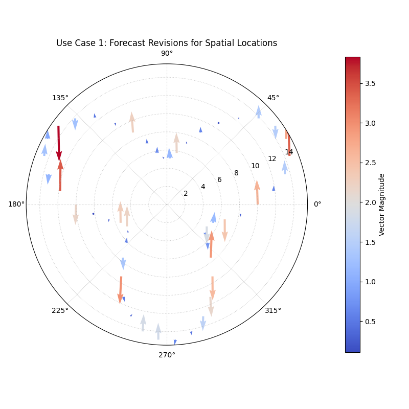
Arrows originating from an initial forecast value, showing the direction and magnitude of the update.

🧠 Analysis and Interpretation

This plot visualizes the stability of a forecast. Each arrow’s base sits on the initial forecast value for a specific location (angle). The arrow itself represents the revision. An arrow pointing outward (a positive radial component) means the forecast was revised upward, while an inward-pointing arrow means it was revised downward. In this example, the revisions appear random and small, with no systematic pattern, suggesting the forecast is relatively stable between updates. A plot with all arrows pointing outward would indicate a systematic upward revision bias.

---

Use Case 2: Mapping a 2D Error Vector Field

Another interesting application is to visualize a model’s error not as a single number, but as a two-dimensional vector. This is common in spatial forecasting, where an error has both a distance component and a directional component.

Imagine a model that predicts the landing location of a weather balloon. The error for each prediction can be described by how many kilometers it was off (radial error) and by which direction it missed (tangential error).

# --- 1. Data Generation: 2D Spatial Errors ---
np.random.seed(42)
n_landings = 60
# The true landing locations
true_r = np.random.uniform(20, 80, n_landings)
true_theta_deg = np.linspace(0, 360, n_landings, endpoint=False)
# Simulate a model that has a systematic drift (e.g., always misses to the "north-east")
radial_error = np.random.normal(2, 2, n_landings)
tangential_error = np.random.normal(5, 2, n_landings)

df_landings = pd.DataFrame({
    'true_dist_km': true_r,
    'true_angle_deg': true_theta_deg,
    'error_radial_km': radial_error,
    'error_tangential_km': tangential_error
})

# --- 2. Plotting the Error Field ---
kd.plot_polar_quiver(
    df=df_landings,
    r_col='true_dist_km',
    theta_col='true_angle_deg',
    u_col='error_radial_km',
    v_col='error_tangential_km',
    theta_period=360,
    title='Use Case 2: Weather Balloon Landing Error Field',
    cmap='viridis',
    scale=150
)

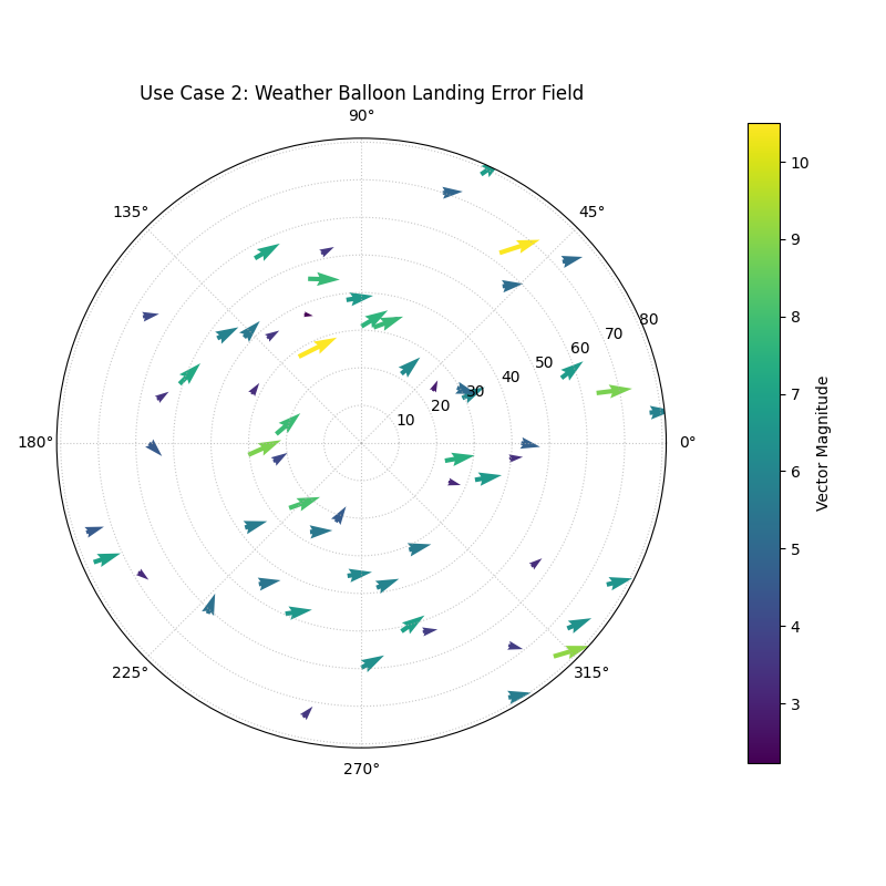
Arrows originating from the true locations, all pointing in a similar direction, revealing a systematic error in the forecast.

🧠 Interpretation

In this plot, the base of each arrow is the true landing location. The arrow itself is the error vector—it points from the true location to the predicted location. A perfect model would have zero- length arrows. Here, we see a clear and problematic pattern: nearly all the arrows point in the same general direction (counter-clockwise and slightly outwards). This reveals a systematic drift in the model. It consistently predicts that the balloons will land further out and further counter-clockwise than they actually do. This is a usefull diagnostic that would be difficult to see without a vector plot.

---

Use Case 3: Comparing Dynamic States with Subplots

One of the most applications of a quiver plot is to compare two different vector fields side-by-side to understand how a dynamic system changes over time or under different conditions. By creating a figure with multiple subplots and passing the individual axes (ax) to the function, we can create a direct and compelling comparative visualization.

Best Practice

For comparative analysis of vector fields, creating a multi-panel figure with matplotlib.pyplot.subplots and then passing each ax object to plot_polar_quiver is the recommended workflow. This gives you full control over the layout and allows for direct, side-by-side comparisons.

Let’s tackle a classic oceanography problem: comparing ocean current patterns between summer and winter.

Practical Example

An oceanographer is studying a regional sea to understand how its circulation patterns change with the seasons. They have collected current velocity data from a network of buoys during both the summer and the winter. They need to visualize and compare these two vector fields to identify seasonal shifts in the direction and speed of the primary currents.

We will create a side-by-side quiver plot. The left panel will show the strong summer currents, and the right panel will show the weaker, more complex winter currents, allowing for an immediate visual assessment of the seasonal change.

# --- 1. Data Generation: Seasonal Ocean Currents ---
np.random.seed(1)
n_buoys = 75
# Buoy positions are the same for both seasons
r_pos = np.random.uniform(10, 50, n_buoys)
theta_pos_deg = np.linspace(0, 360, n_buoys, endpoint=False)

# Summer: Strong, consistent counter-clockwise gyre
u_summer = np.random.normal(0, 0.1, n_buoys)
v_summer = 2.0 + np.sin(np.deg2rad(theta_pos_deg)) * 0.5
df_summer = pd.DataFrame({
    'dist_km': r_pos, 'angle_deg': theta_pos_deg,
    'u_rad': u_summer, 'v_tan': v_summer
})

# Winter: Weaker, less consistent flow
u_winter = np.random.normal(0, 0.2, n_buoys)
v_winter = 0.8 - np.sin(np.deg2rad(theta_pos_deg)) * 0.5 # Weaker, different pattern
df_winter = pd.DataFrame({
    'dist_km': r_pos, 'angle_deg': theta_pos_deg,
    'u_rad': u_winter, 'v_tan': v_winter
})

# --- 2. Create a figure with two polar subplots ---
fig, (ax1, ax2) = plt.subplots(1, 2, figsize=(18, 9),
                             subplot_kw={'projection': 'polar'})

# --- 3. Plot each season on its dedicated axis ---
kd.plot_polar_quiver(
    df=df_summer, ax=ax1, r_col='dist_km', theta_col='angle_deg',
    u_col='u_rad', v_col='v_tan', theta_period=360,
    title='Summer Current Field', cmap='plasma', scale=40
)
kd.plot_polar_quiver(
    df=df_winter, ax=ax2, r_col='dist_km', theta_col='angle_deg',
    u_col='u_rad', v_col='v_tan', theta_period=360,
    title='Winter Current Field', cmap='cividis', scale=40
)

fig.suptitle('Use Case 3: Seasonal Comparison of Ocean Currents', fontsize=16)
# fig.tight_layout(rect=[0, 0.03, 1, 0.95]) # handled by kd.savefig
kd.savefig("gallery/images/gallery_polar_quiver_seasonal.png", close=True)

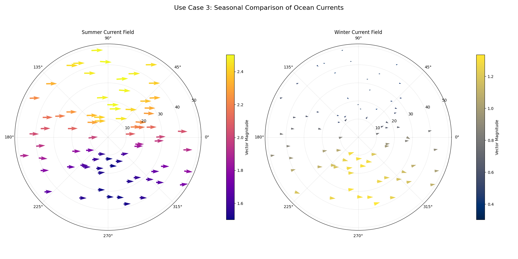
A two-panel figure showing a strong, bright, and coherent rotational current in the summer (left) and a weaker, darker, and less organized current in the winter (right).

🧠 Interpretation

The side-by-side comparison immediately highlights the dramatic seasonal shift in ocean circulation. The Summer plot (left) displays a strong, coherent, counter-clockwise gyre, with the bright yellow and orange arrows indicating high-velocity currents throughout the northern half of the region. In stark contrast, the Winter plot (right) shows a much weaker and less organized system. The arrows are predominantly dark purple and blue, indicating a significant drop in current speed, and the cohesive rotational pattern has partially broken down. This comparative view provides an intuitive summary of the system’s seasonal dynamics.

---

For a deeper understanding of the mathematical concepts behind vector fields and their visualization, you may refer to the main Visualizing Vector Fields (plot_polar_quiver()) section.