Spatial Diagnostic Plots Gallery

This gallery showcases the complete suite of spatial and polar diagnostic functions from kdiagram.plot.spatial. The module bridges the gap between classical tabular forecast evaluation and geographic insight: every plot here works with any (x, y) or (longitude, latitude) coordinate system — no basemap library required.

The examples are built around a synthetic land-subsidence monitoring network of 120 wells distributed across a coastal urban–peri-urban–rural gradient (modelled after the Zhongshan, China dataset used in the k-diagram paper). Two Gaussian hotspots in the south create elevated prediction-interval widths and reduced coverage, giving every plot a non-trivial spatial pattern to reveal.

Note

All code can be run locally. Save paths in savefig= must be adjusted to your output directory. Images are referenced from ../images/spatial/ relative to this file.

---

Spatial Scatter Plot

The plot_spatial_scatter() function maps any numeric metric onto a scatter of geographic coordinates. It is the starting point for spatial forecast evaluation: where is the model good, and where does it fail?

Plot Anatomy

• Position (x, y): Geographic or projected coordinates — longitude and latitude in the examples below, but any consistent unit works.

• Color: The primary metric encoded on the colormap. Cold colors indicate low values; warm/bright colors indicate high values.

• Marker size (optional): A second numeric column can control bubble area, enabling two-dimensional spatial encoding.

• Colorbar: A vertical bar on the right gives the numeric scale.

---

Use Case 1: Where is the anomaly severity highest?

The simplest and most frequent use is coloring each monitoring station by a single scalar metric — here the anomaly severity score. High-severity clusters immediately reveal geographic regions the model struggles with.

import kdiagram as kd
import numpy as np
import pandas as pd

rng = np.random.default_rng(2024)
N = 120
# ... (build df with 'lon', 'lat', 'severity' columns)

ax = kd.plot_spatial_scatter(
    df, "lon", "lat", "severity",
    cmap="hot_r", vmin=0, vmax=4.5,
    s=55, alpha=0.88,
    colorbar_label="Anomaly Severity Score",
    title="Spatial Distribution of Forecast Anomaly Severity (H1)",
    xlabel="Longitude (degrees E)",
    ylabel="Latitude (degrees N)",
)

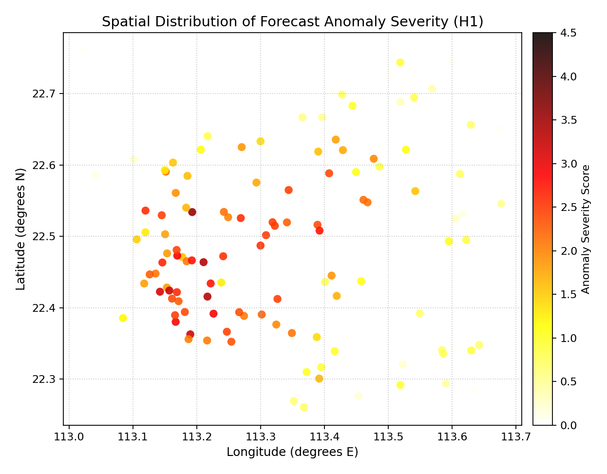
Hot colors (yellow/white) mark the two high-severity hotspots in the southern urban zone. Northern rural stations are dark (low severity).

Analysis and Interpretation

The plot immediately reveals two distinct hotspots in the south: one near (113.20, 22.42) and another at (113.45, 22.52), corresponding to the two Gaussian severity peaks injected into the data. The northern peri-urban and rural stations show much lower severity, suggesting the model degrades in areas of high urban land-use intensity. This spatial concentration would be completely invisible in an aggregate coverage score.

---

Use Case 2: Coverage rate and interval width in one view

By mapping coverage rate to color and interval width to bubble size, two critical uncertainty dimensions are encoded simultaneously. A station with a small bubble (narrow interval) and red color (low coverage) is the most dangerous combination — the model is falsely confident.

ax = kd.plot_spatial_scatter(
    df, "lon", "lat", "coverage",
    size_col="width_h1",
    size_range=(15, 350),
    cmap="RdYlGn", vmin=0.6, vmax=1.0,
    alpha=0.82, edgecolor="0.3", linewidths=0.4,
    colorbar_label="Empirical Coverage Rate",
    title="Coverage Rate (color) vs Interval Width (size) per Station",
    xlabel="Longitude (degrees E)",
    ylabel="Latitude (degrees N)",
)

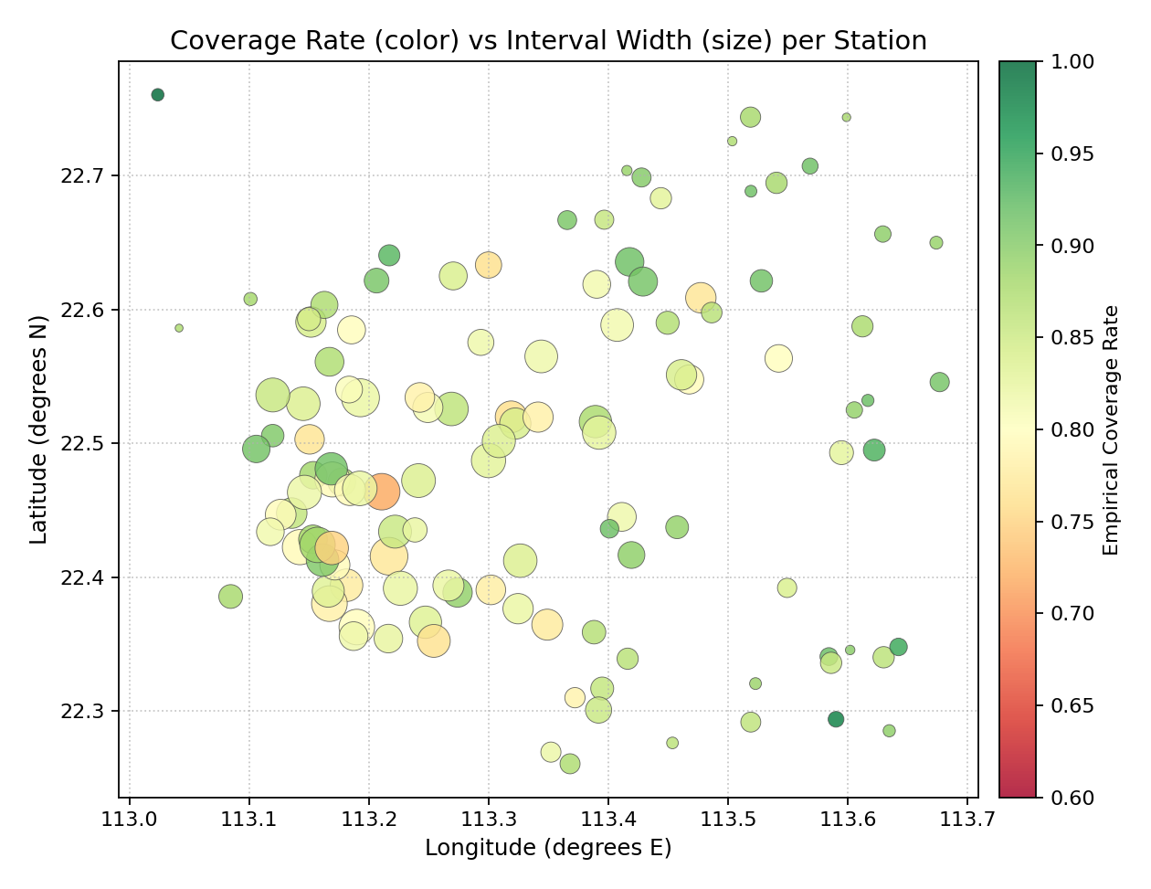
Large green bubbles (north) = wide intervals with good coverage. Small red bubbles (south) = narrow intervals that still under-cover — the riskiest calibration profile.

Analysis and Interpretation

Southern stations combine small size (narrow prediction intervals) with red color (below-nominal coverage), confirming that the model is overconfident in the high-subsidence zone. Northern stations are well-calibrated: wide intervals (large bubbles) with coverage rates near or above the 90% nominal (green). Stations whose bubble is large and red (over-wide AND under-covering) would indicate a different failure mode — the model is simultaneously imprecise and unreliable — none appear here, suggesting the failure is one of overconfidence, not imprecision.

---

Spatial Heatmap

The plot_spatial_heatmap() function interpolates the scattered station observations onto a regular 2-D grid using scipy.interpolate.griddata and displays the result as a continuous color surface. This reveals the spatial field underlying the point measurements, making gradients and transition zones visible.

Plot Anatomy

• Continuous surface: Interpolated from the scattered point values. Regions with dense stations are well-constrained; the surface may become less reliable near the edges where stations are sparse.

• Scatter overlay: Optional dots (scatter_overlay=True) show the exact station locations, helping the reader judge where the surface is observation-supported vs. extrapolated.

• Iso-contours: Optional level lines (contour=True) draw boundaries between equal-metric zones. Useful for zoning decisions.

---

Use Case 1: Smooth severity field — identifying spatial gradients

The cubic method produces a smooth, differentiable surface that is ideal for identifying broad spatial gradients and hotspot boundaries.

ax = kd.plot_spatial_heatmap(
    df, "lon", "lat", "severity",
    method="cubic", resolution=250,
    contour=False,
    scatter_overlay=True,
    scatter_s=18, scatter_color="white", scatter_alpha=0.55,
    cmap="hot_r", vmin=0, vmax=4.5,
    colorbar_label="Anomaly Severity Score",
    title="Interpolated Severity Surface (H1) - Cubic Method",
    xlabel="Longitude (degrees E)",
    ylabel="Latitude (degrees N)",
)

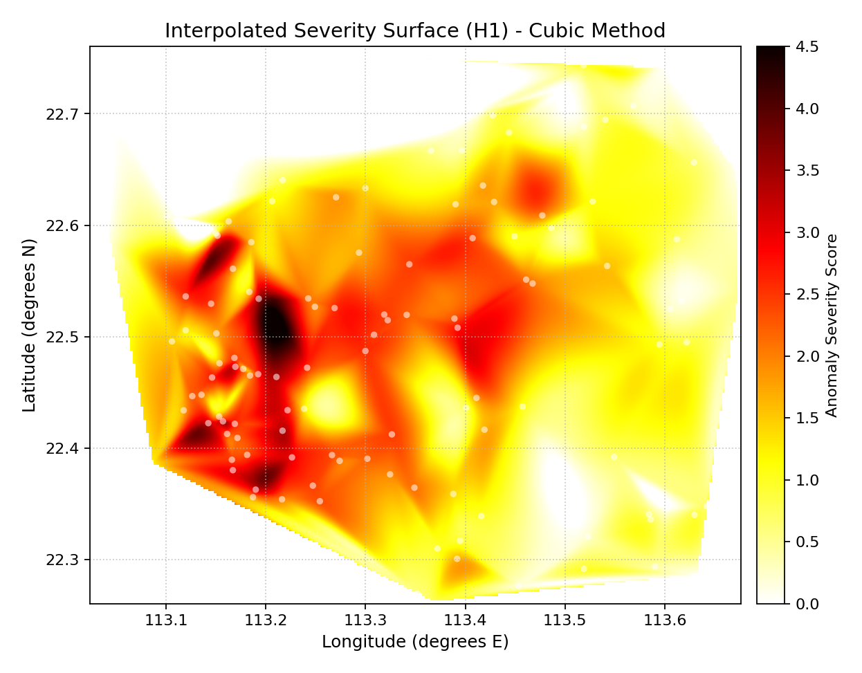
The cubic surface clearly delineates the two hotspot zones as bright islands. White dots confirm that the surface is well-supported by observations throughout the domain.

Analysis and Interpretation

The continuous surface makes spatial gradients visible that the scatter plot can only imply: the two hotspots show a smooth peak (not a sharp discontinuity), suggesting the underlying severity is spatially autocorrelated — nearby wells share similar model failure profiles. The white-dot overlay confirms that the interpolation is well- constrained everywhere: there are no large un-observed voids.

---

Use Case 2: Horizon H7 width with iso-contours — zoning for infrastructure

Iso-contour lines divide the domain into discrete width zones, directly translating the heatmap into actionable geographic boundaries (e.g., “Zone A: width > 4 m — elevated monitoring priority”).

ax = kd.plot_spatial_heatmap(
    df, "lon", "lat", "width_h7",
    method="linear", resolution=220,
    contour=True, contour_levels=7,
    contour_color="white", contour_linewidth=0.9,
    scatter_overlay=True, scatter_s=12,
    cmap="plasma", vmin=0, vmax=6,
    colorbar_label="Interval Width H7 (m)",
    title="H7 Interval Width Surface with Iso-Contours",
    xlabel="Longitude (degrees E)",
    ylabel="Latitude (degrees N)",
)

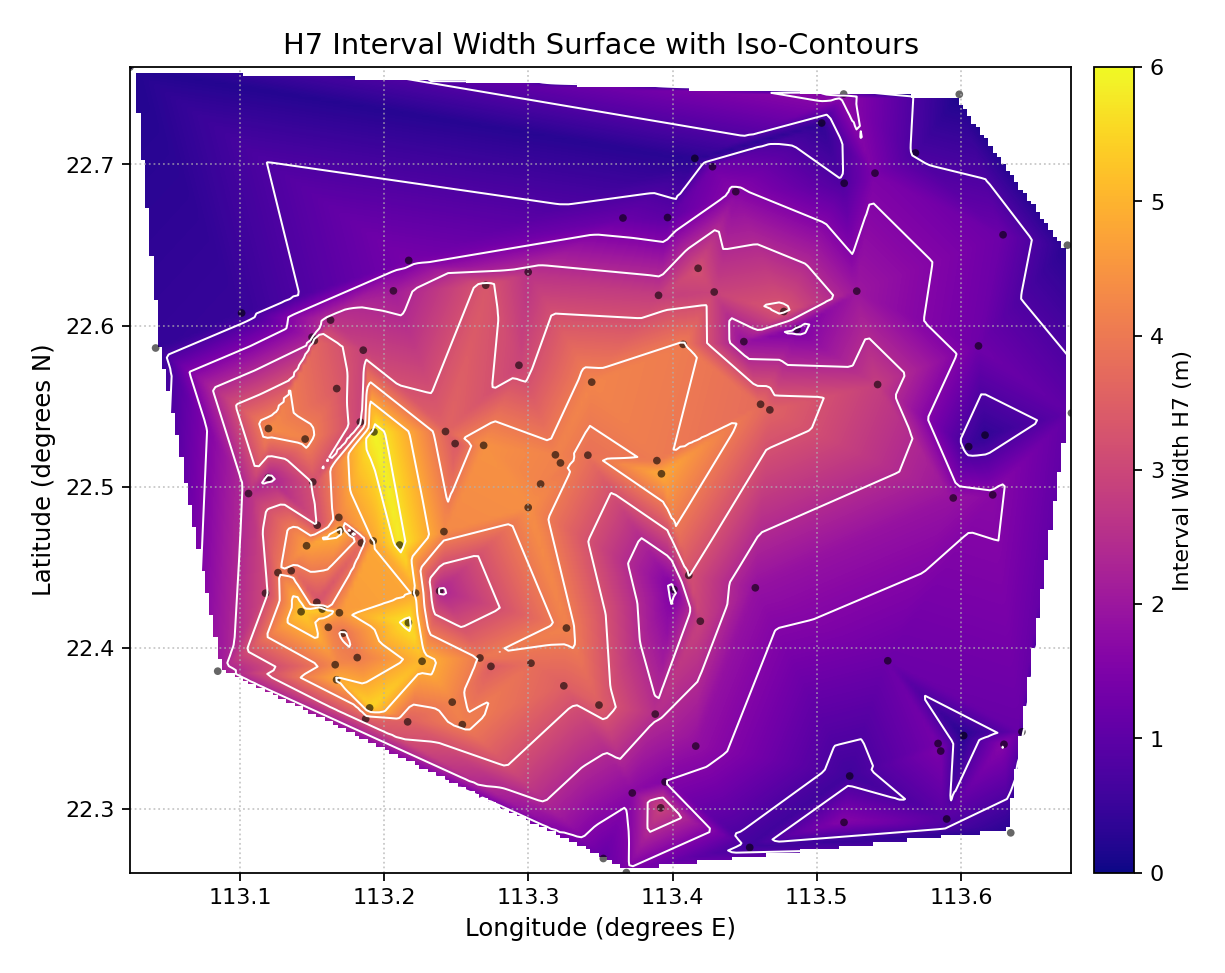
Plasma colormap + white contour lines divide the domain into 7 uncertainty bands. The innermost bright zone marks the highest-uncertainty core.

Analysis and Interpretation

With seven contour levels the heatmap becomes a risk-zone map: a decision-maker can immediately identify which stations fall inside the highest-uncertainty envelope (bright yellow core) vs. the low-uncertainty periphery (dark purple). The contour spacing is also informative — closely-spaced contours in the north indicate a steep transition from low to moderate uncertainty, while the well-spaced contours around the southern hotspot show a more gradual gradient. The H7 surface is notably broader and brighter than H1, confirming that forecast uncertainty grows with horizon across the entire domain.

---

Spatial Uncertainty Map

The plot_spatial_uncertainty() function aggregates multiple time steps per station and produces a bubble map that simultaneously shows two key uncertainty diagnostics:

• Bubble size — the mean prediction-interval width at that location.

• Bubble color — the deviation of the empirical coverage rate from the nominal level (e.g., 90%).

Plot Anatomy

• Large bubbles → wide prediction intervals (high uncertainty).

• Small bubbles → narrow intervals (high sharpness — but also high risk if coverage is low).

• Blue/cool color → over-coverage (intervals too wide for the nominal level; conservative model).

• Red/warm color → under-coverage (intervals too narrow; the model is overconfident at this station).

• White/neutral color → coverage close to the nominal level (well-calibrated).

---

Use Case 1: Global uncertainty overview — width vs. coverage deviation

This is the most informative single-plot summary of a probabilistic forecast evaluated over a spatial network.

# df_ts: long-format DataFrame with one row per (station, timestep)
ax = kd.plot_spatial_uncertainty(
    df_ts, "lon", "lat", "actual", "q10", "q90",
    nominal=0.90,
    cmap="RdBu_r",
    size_range=(20, 450),
    alpha=0.83,
    title="Uncertainty Map: Width (size) vs Coverage Deviation (color)",
    xlabel="Longitude (degrees E)",
    ylabel="Latitude (degrees N)",
)

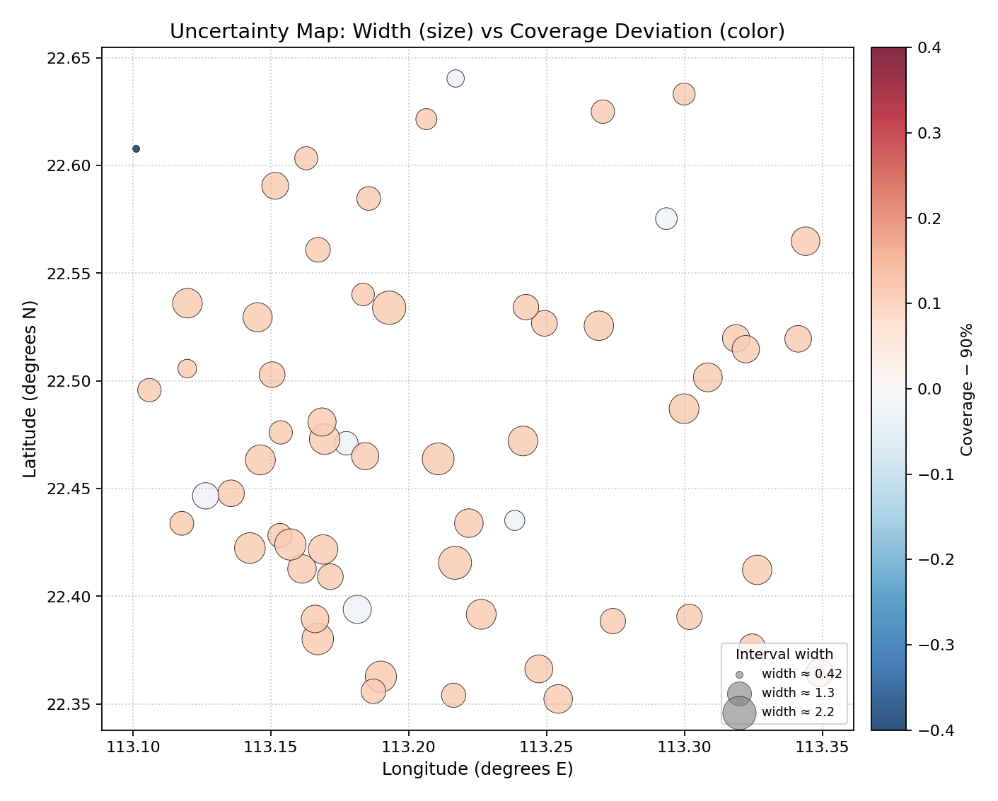
Red = under-coverage (overconfident station); blue = over-coverage (conservative); large bubble = wide interval. Southern stations are red and have small-to-medium bubbles — the dangerous overconfident cluster.

Analysis and Interpretation

The ideal station would have white color (correct coverage) and moderate size (reasonable sharpness). The southern cluster shows red + small-to-medium bubbles — the model is overconfident: the intervals are narrow and still fail to cover the true value at the nominal rate. Northern stations are closer to white/blue, indicating conservative but well-calibrated forecasts. This plot answers in one glance: “Is the calibration failure geographic, and does it coincide with the model being sharp or wide?”

---

Use Case 2: Diagnosing a southern under-coverage hotspot

By amplifying the coverage deficit in southern stations, the plot isolates the overconfident cluster and makes the geographic boundary of the failure zone clearly visible.

# Tighten intervals for southern stations to amplify the hotspot
df_ts3 = df_ts.copy()
south_mask = df_ts3["lat"] < 22.50
df_ts3.loc[south_mask, "q90"] -= 0.5   # shrink upper bound

ax = kd.plot_spatial_uncertainty(
    df_ts3, "lon", "lat", "actual", "q10", "q90",
    nominal=0.90,
    cmap="coolwarm",
    size_range=(25, 500),
    alpha=0.80,
    title="Southern Hotspot: Under-Coverage Cluster Revealed",
    xlabel="Longitude (degrees E)",
    ylabel="Latitude (degrees N)",
)

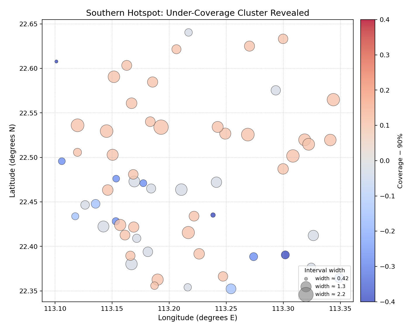
The southern under-coverage cluster is now clearly separated (red, small) from the northern over-coverage zone (blue, larger). The transition zone in the middle is visible as white stations.

Analysis and Interpretation

The coolwarm diverging colormap centered at zero coverage deviation makes the geographic split immediately legible: a crisp north–south boundary near latitude 22.50 separates the overconfident red south from the conservative blue north. A risk-management team could use this boundary to define different monitoring protocols for each zone.

---

Spatial Coverage Map

The plot_spatial_coverage() function maps pre-computed coverage rates (one value per station, already aggregated externally) onto a scatter using a diverging colormap centered on the nominal level. An optional tolerance parameter flags stations that exceed an acceptable deviation with a star marker.

Plot Anatomy

• Color (diverging): Blue = above-nominal coverage (conservative model); red = below-nominal (overconfident); white = exactly nominal.

• Star overlay (annotate=True):** Stations outside the tolerance band are additionally marked with a star to draw attention.

• Colorbar: Centered on the nominal level; the color scale spans deviations in both directions.

---

Use Case 1: Network-wide coverage audit against the 90% nominal

A single map reveals which stations the model fails to cover at the contracted reliability level and by how much.

ax = kd.plot_spatial_coverage(
    df, "lon", "lat", "coverage",
    nominal=0.90,
    cmap="RdBu",
    s=70, alpha=0.88,
    title="Coverage Rate Deviation from 90% Nominal",
    xlabel="Longitude (degrees E)",
    ylabel="Latitude (degrees N)",
)

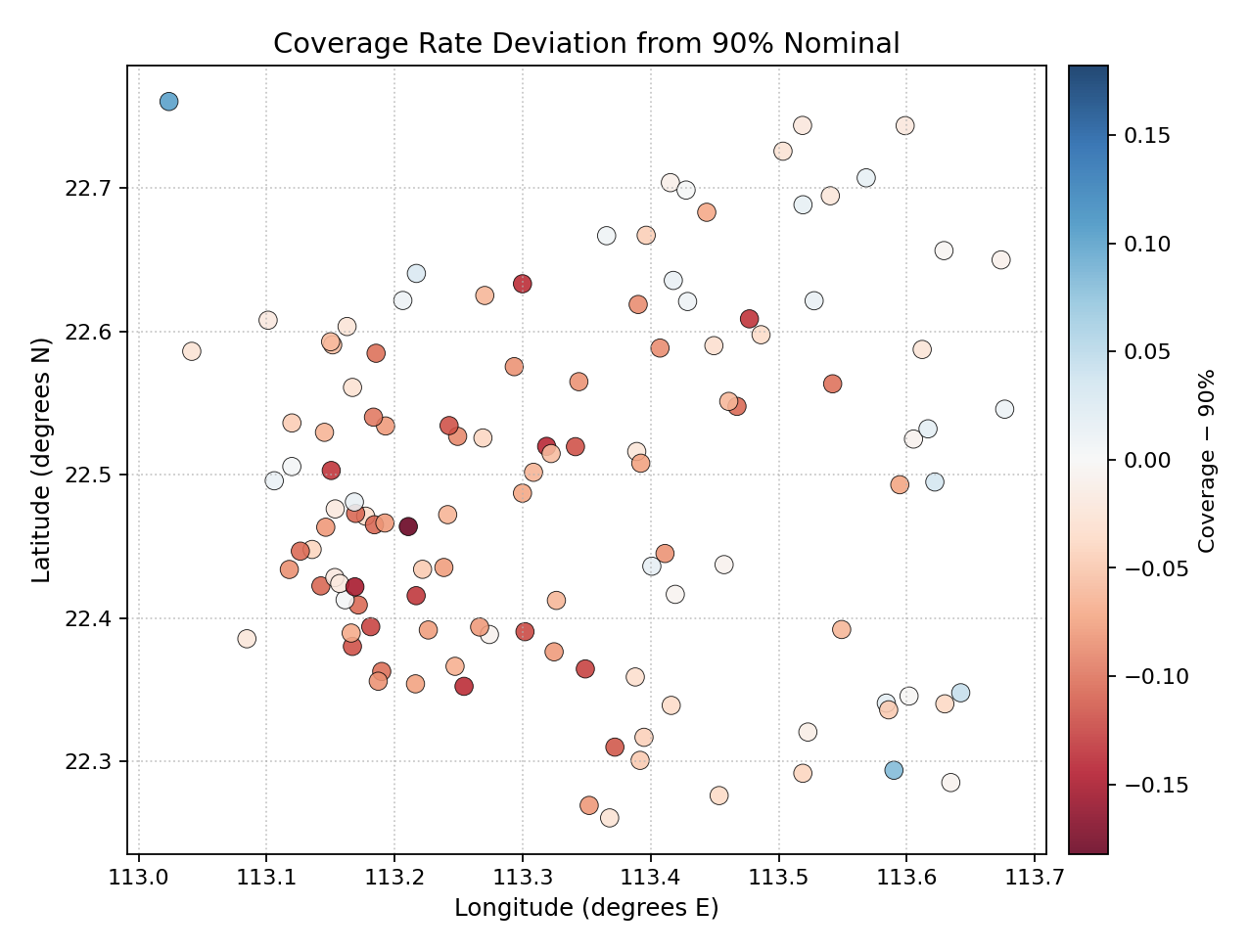
Red stations (south) are under-covered; blue stations (north) are over-covered. The white band in the middle marks the well-calibrated transition zone.

Analysis and Interpretation

The diverging colormap centered on 90% makes deviations in both directions equally legible. The southern cluster is strongly red, indicating systematic under-coverage (the model is overconfident in the high-severity zone). The northern rural stations lean blue (slightly over-conservative), but remain close to the nominal. No station is perfectly white, confirming that perfect spatial calibration is rarely achieved in practice.

---

Use Case 2: Flagging stations that violate a contractual tolerance

In operational settings a ±8% tolerance is often contractually defined. Setting tol=0.08 adds a star marker to every station outside this band, making compliance audits immediate.

ax = kd.plot_spatial_coverage(
    df, "lon", "lat", "cov_xtft",   # XTFT model coverage
    nominal=0.90, tol=0.08,
    cmap="RdBu",
    s=65, alpha=0.85,
    annotate=True,
    title="XTFT Coverage: Stations Outside +-8% Tolerance Flagged",
    xlabel="Longitude (degrees E)",
    ylabel="Latitude (degrees N)",
)

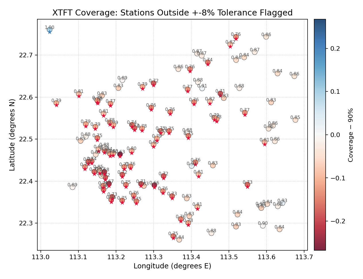
Star markers identify the XTFT stations that violate the +-8% tolerance. The stars cluster in the south, confirming that the coverage failures are geographically concentrated.

Analysis and Interpretation

The annotate=True flag immediately highlights which stations require action: those with stars must either have their prediction intervals recalibrated or be flagged for manual review. The geographic concentration of flagged stations (south) directs the recalibration effort precisely — rather than retraining the entire model, a spatially-adaptive post-processing step targeting the southern zone may be sufficient.

---

Multi-Model Spatial Comparison

The plot_spatial_comparison() function produces an N-panel grid, one panel per model or condition, all on a shared color scale. It is the standard way to answer: “Which model has the lowest interval width everywhere? Are the improvements geographically uniform?”

Plot Anatomy

• Panel grid: One panel per model/condition. Layout controlled by ncols.

• Shared colorbar: A single colorbar (right-most column) applies to all panels when shared_scale=True, making cross-panel comparisons rigorous.

• Panel titles: Derived from the names list or the raw column name if not provided.

---

Use Case 1: Three-model H1 interval width comparison

Side-by-side maps answer at a glance: “Which model produces the narrowest prediction intervals, and is the improvement geographically uniform?”

axes = kd.plot_spatial_comparison(
    df, "lon", "lat",
    metric_cols=["width_qar", "width_qgbm", "width_xtft"],
    names=["QAR", "QGBM", "XTFT"],
    ncols=3, shared_scale=True,
    cmap="plasma", s=45, alpha=0.85,
    colorbar_label="Interval Width H1 (m)",
)

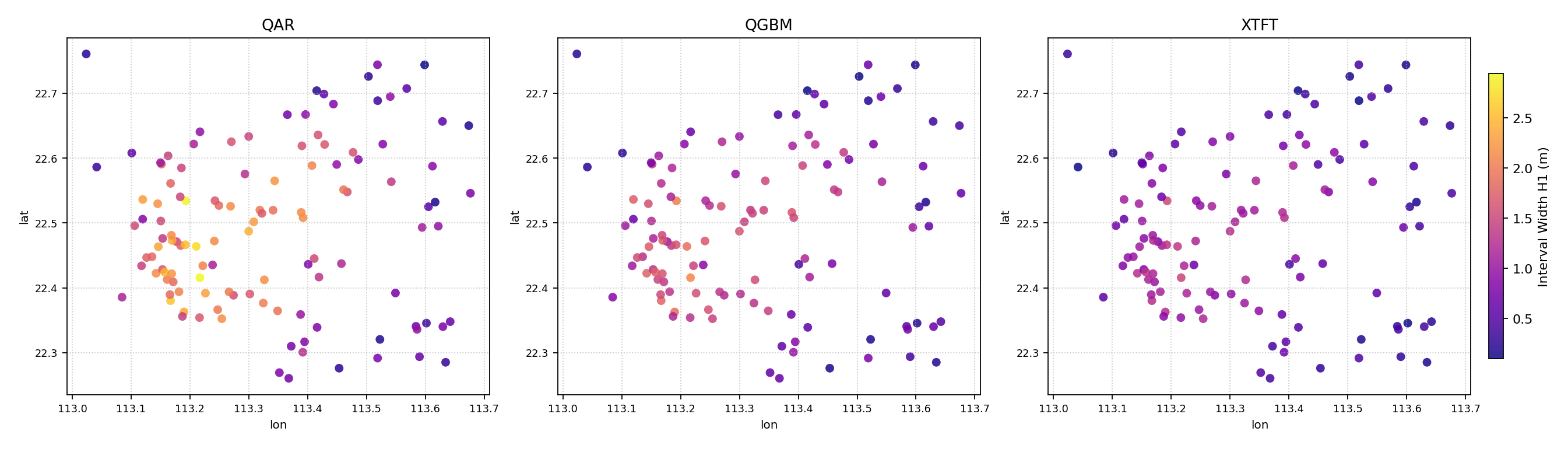
Left to right: QAR (wide, high coverage), QGBM (balanced), XTFT (narrow, sharp). The hotspot geometry is identical across all three models, but the color intensity scales down from left to right, confirming XTFT is consistently sharper.

Analysis and Interpretation

All three panels share the same hotspot geometry in the south, confirming that the geographic challenge is model-agnostic — these wells are hard to forecast for any model. But the color intensity drops systematically from QAR → QGBM → XTFT, proving that XTFT achieves uniformly sharper intervals without introducing new geographic biases. A model that achieved sharpness gains only in the north (easy zone) while remaining wide in the south would show a different pattern.

---

Use Case 2: Horizon evolution — does uncertainty grow uniformly?

Using metric_cols as a list of horizon columns reveals whether the model’s uncertainty growth is spatially uniform or concentrated in specific areas.

axes = kd.plot_spatial_comparison(
    df, "lon", "lat",
    metric_cols=["width_h1", "width_h3", "width_h5", "width_h7"],
    names=["H1", "H3", "H5", "H7"],
    ncols=2, shared_scale=True,
    cmap="viridis", s=40, alpha=0.85,
    colorbar_label="Interval Width (m)",
)

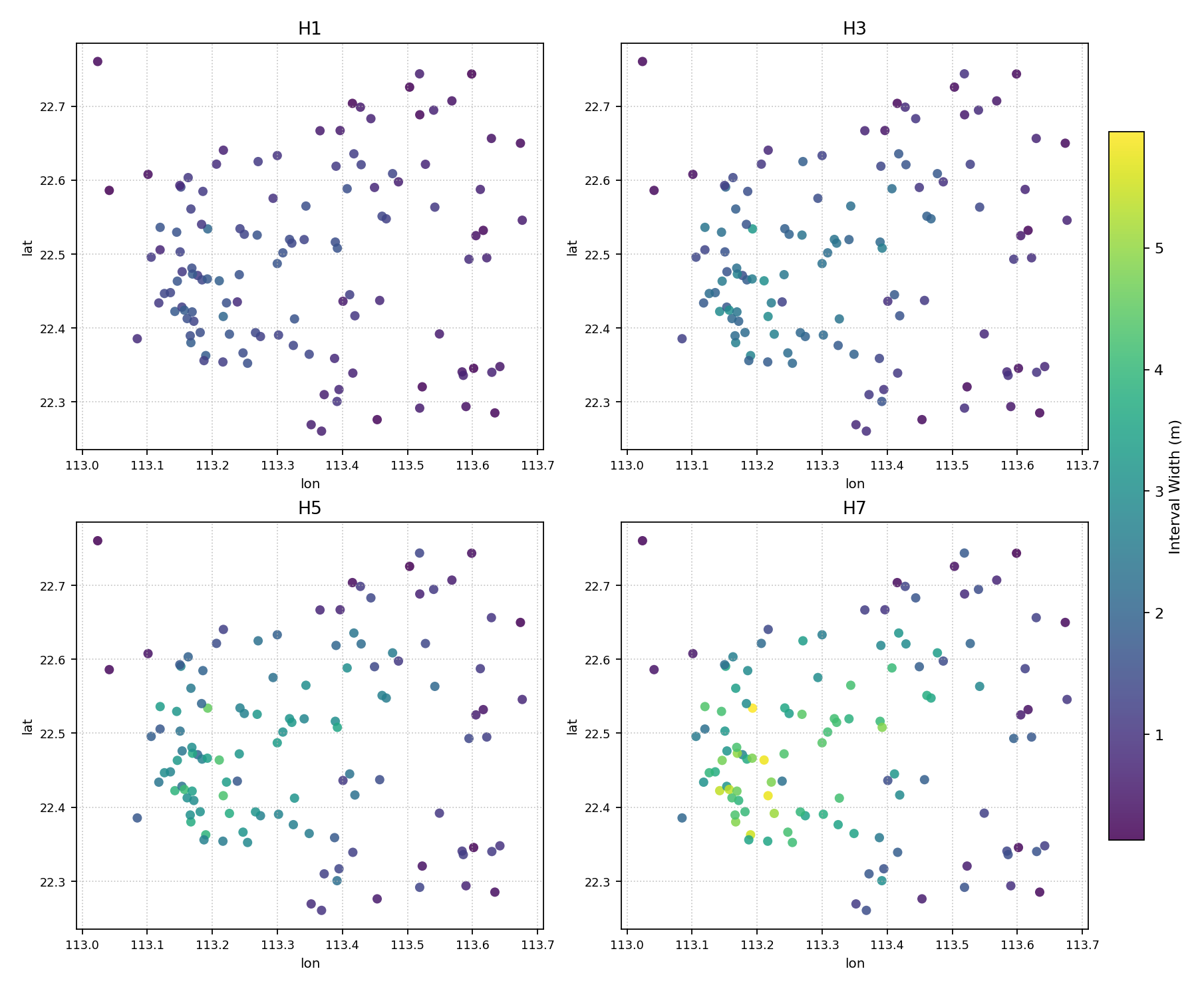
Top row: H1 (narrow) and H3; bottom: H5 and H7 (wide). The southern hotspot grows brighter with horizon, showing that uncertainty amplifies most in the already-difficult zone.

Analysis and Interpretation

The four panels tell a complete uncertainty story. At H1 the domain is mostly dark (narrow intervals) with only a faint hotspot in the south. By H7 the southern hotspot dominates — the brighter colors confirm that uncertainty growth is spatially non-uniform: it amplifies fastest in the already-difficult zone. A spatially uniform uncertainty growth would produce panels where all regions brighten proportionally; instead the south brightens faster, signalling a geographic interaction between forecast horizon and model accuracy.

---

Geographic Ordering Map

The plot_spatial_ordering() function renders the site ordering that underpins the polar diagnostics. Sites are ranked 0 → N−1 by a geographic criterion (latitude, longitude, or any custom column) and color-coded by that rank. Optional arrows trace the traversal path so the reader can follow the ordering across the domain.

This plot is the key to reading the polar hedgehog diagrams: it answers the question “which geographic location corresponds to which polar angle?”

Plot Anatomy

• Color (sequential): Encodes rank — dark = first site (rank 0), bright = last site (rank N−1).

• Arrows: Connect consecutive sites in rank order. Arrow density is controlled by arrow_step (default N//15).

• Annotations: The label_sites list marks a subset of sites with their 1-based rank number, giving the polar plots a look-up key.

---

Use Case 1: South-to-north ordering by latitude

The default ordering traverses the domain from the southernmost station (rank 0, polar angle ~0°) to the northernmost (rank N−1, polar angle ~360°).

ax = kd.plot_spatial_ordering(
    df, "lon", "lat",
    order_by="lat", order_ascending=True,
    show_arrows=True, arrow_step=8,
    label_sites=[0, 29, 59, 89, 119],
    colorbar_label="Site order (0 = southernmost)",
    title="Geographic Domain: Site Ordering (South to North)",
    xlabel="Longitude (degrees E)",
    ylabel="Latitude (degrees N)",
)

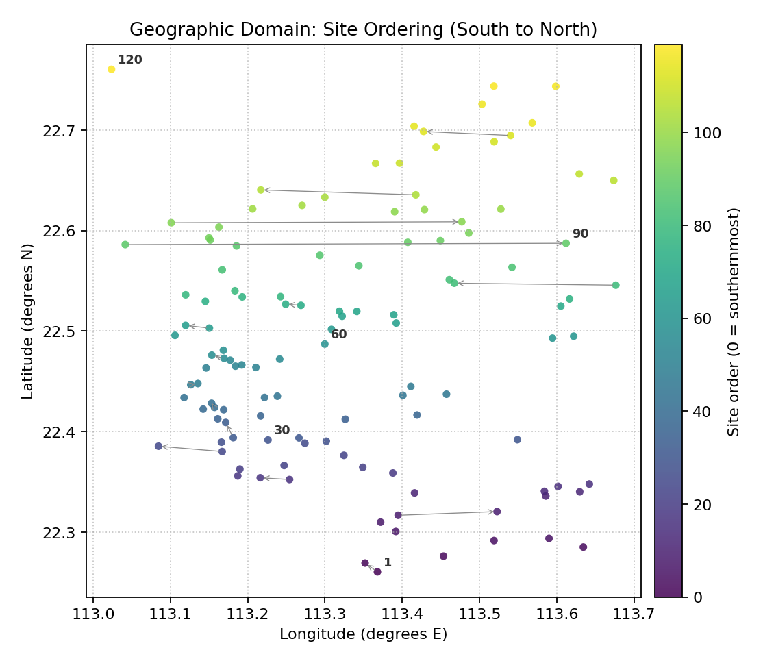
Dark (low rank) stations are southernmost; bright (high rank) are northernmost. Arrows trace the monotonic south-to-north traversal. Labeled stations 1, 30, 60, 90, 120 map to polar angles 0, pi/2, pi, 3*pi/2, 2*pi respectively.

Analysis and Interpretation

A smooth color gradient from south to north confirms that the ordering faithfully captures the latitudinal structure of the network. Any color jump (a dark station embedded in a bright cluster) would indicate a station that is geographically isolated from its ranked neighbors — worth noting when interpreting gaps in the polar hedgehog. The labeled sites provide the exact polar-angle look-up for the hedgehog diagrams: station 60 (rank 59) maps to polar angle \(\approx \pi\) (the left side of the hedgehog circle).

---

Use Case 2: West-to-east ordering by longitude

Switching to order_by="lon" redefines the polar angle assignment and produces a completely different polar diagnostic — useful for comparing the structure of the metric in the two orthogonal spatial directions.

ax = kd.plot_spatial_ordering(
    df, "lon", "lat",
    order_by="lon", order_ascending=True,
    show_arrows=True, arrow_step=8,
    cmap="plasma",
    label_sites=[0, 39, 79, 119],
    colorbar_label="Site order (0 = westernmost)",
    title="Geographic Domain: Site Ordering (West to East)",
    xlabel="Longitude (degrees E)",
    ylabel="Latitude (degrees N)",
)

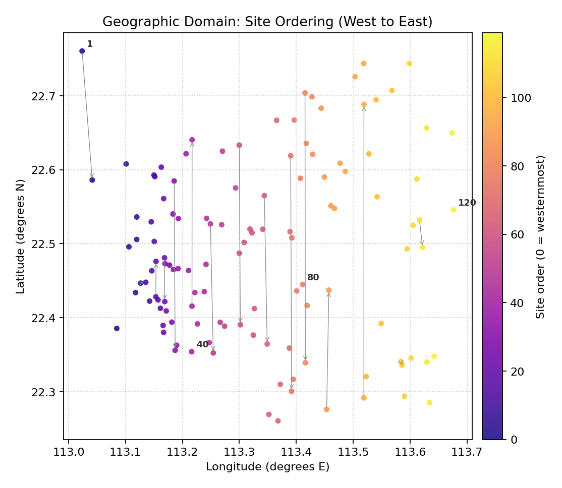
Plasma colormap; dark = west, bright = east. Arrows cross latitude bands, producing a zigzag traversal rather than the monotonic sweep seen in the latitude ordering.

Analysis and Interpretation

With longitude ordering the arrows cross latitude bands, indicating that the traversal zigzags across the domain. This matters for the polar diagnostic: in the latitude-ordered hedgehog adjacent spikes correspond to geographically adjacent sites; in the longitude-ordered hedgehog adjacent spikes may be far apart in latitude. Comparing the two hedgehogs helps distinguish whether a metric cluster is primarily a north–south phenomenon or an east–west one.

---

Polar Hedgehog Diagnostic

The plot_polar_from_spatial() function is the central visualization of the spatial-polar framework. Each site is represented as a radial spike (needle) on a polar plot:

• Angle (\(\theta_i = 2\pi i / N\)) encodes the geographic rank.

• Radius encodes the metric value at that site.

Long spikes mark high-metric sites; the angular position tells you where those sites are in the ordering, and by consulting the companion ordering map you know where they are geographically.

A second mode (ring mode, via horizon_cols) places concentric rings for multiple horizons or conditions, enabling simultaneous comparison across the full ordering spectrum.

Plot Anatomy

• Spike angle: Geographic rank → polar angle. North (top) = rank 0 (first site); the angle increases clockwise by default.

• Spike length (radius): Metric value. Longer = higher metric.

• Spike color (single-horizon): A second column, or the metric itself, drives the colormap.

• Reference rings: Faint dashed circles at regular radii help read absolute metric values.

• Ring labels (ring mode): The label for each concentric ring is placed at a fixed angle for quick identification.

---

Use Case 1: Severity hedgehog — where is the model worst?

This is the primary use: a compact 360° summary of how severity is distributed across the ordered sites. A cluster of long spikes in one angular arc reveals a geographic concentration of forecast failures.

ax = kd.plot_polar_from_spatial(
    df, "lon", "lat", "severity",
    order_by="lat",
    cmap="hot_r",
    n_ring_labels=4,
    colorbar_label="Anomaly Severity Score",
    title="Polar Diagnostic: Severity Distribution Across Ordered Sites",
)

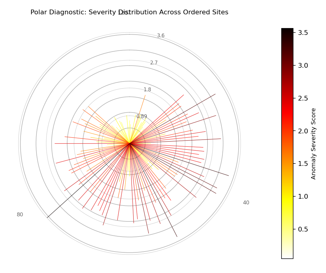
Long, bright spikes in the lower arc (ranks 0-40, southern sites) confirm that severity is concentrated in the south. Northern sites (top arc) have short, dark spikes — the model performs well there.

Analysis and Interpretation

With latitude ordering, ranks 0-40 map to the lower half of the polar circle (angles 0 to ~120°). The concentration of long bright spikes in that angular region directly confirms the southern severity hotspot seen in the scatter map. The pattern is not symmetric around the circle — a symmetric hedgehog would indicate spatially uniform severity. The visible arc-length of the long-spike cluster also tells you its geographic extent: an arc spanning ~90° means the hotspot covers roughly 25% of the stations.

---

Use Case 2: Multi-horizon ring encoding H1 → H7

By passing horizon_cols the function switches to ring mode: each ring corresponds to one forecast horizon, stacked outward from the center. This allows the evolution of uncertainty with horizon to be read at every site simultaneously.

ax = kd.plot_polar_from_spatial(
    df, "lon", "lat", "width_h1",
    horizon_cols=["width_h3", "width_h5", "width_h7"],
    horizon_labels=["H1", "H3", "H5", "H7"],
    horizon_colors=["#4393c3", "#f4a582", "#d6604d", "#a50026"],
    order_by="lat",
    title="Multi-Horizon Ring: Uncertainty Growth from H1 (inner) to H7 (outer)",
)

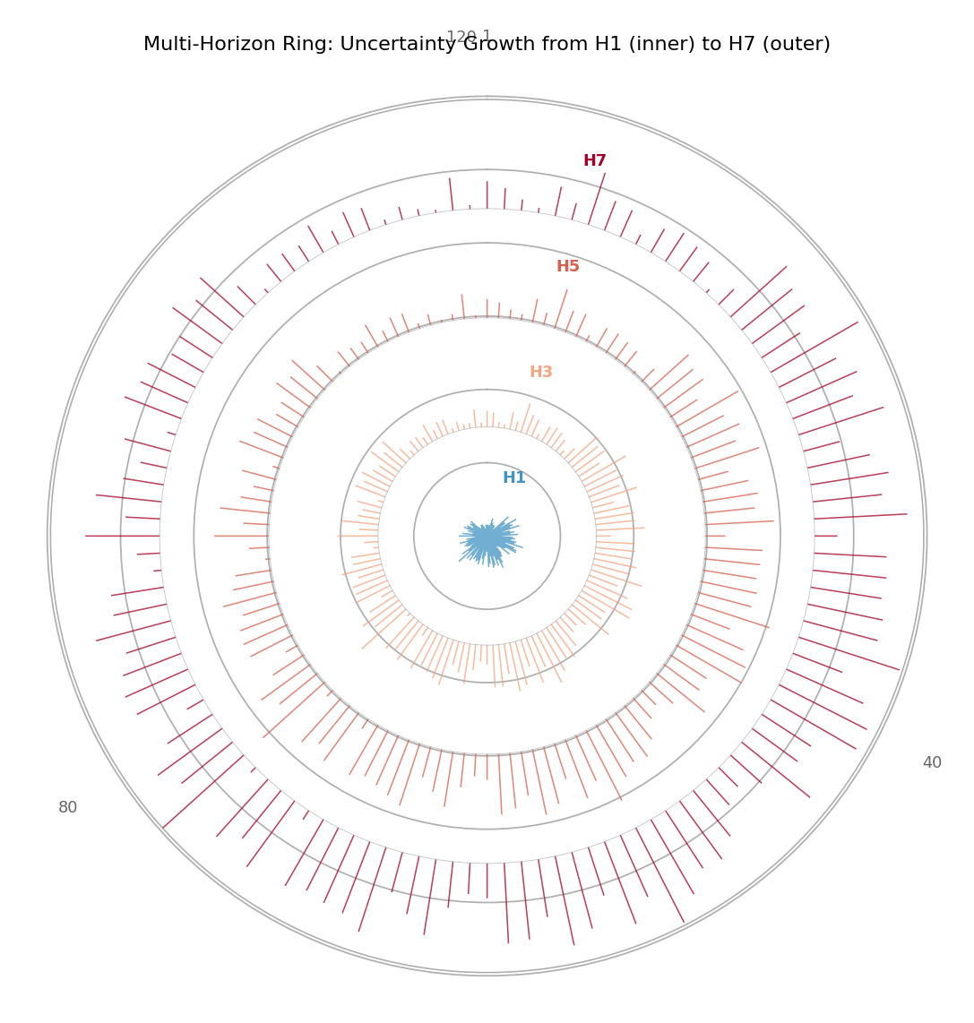
Four concentric rings: H1 (innermost blue) to H7 (outermost red). The southern arc shows the largest radial growth from H1 to H7 — uncertainty amplifies most where the model is already weakest.

Analysis and Interpretation

Reading this diagram at a single angle (site) traces the horizon profile of uncertainty for that location. Sites in the southern arc show large radial growth: the H7 spike extends much further than the H1 spike, indicating rapidly growing uncertainty with horizon. Northern sites show smaller, more uniform rings — the uncertainty still grows, but proportionally less. This confirms a spatially non-uniform horizon sensitivity: long-horizon forecasts are especially unreliable in the high-severity zone.

---

Use Case 3: Decoupled color and radius — severity on width spikes

Setting color_col to a different column from metric_col encodes two independent spatial patterns on the same hedgehog: spike length shows one metric (interval width) while spike color shows another (anomaly severity).

ax = kd.plot_polar_from_spatial(
    df, "lon", "lat", "width_h1",
    color_col="severity",         # severity drives color
    order_by="lat",
    cmap="RdYlGn_r",
    colorbar_label="Anomaly Severity (color)",
    title="Polar Diagnostic: Width (radius) vs Severity (color)",
)

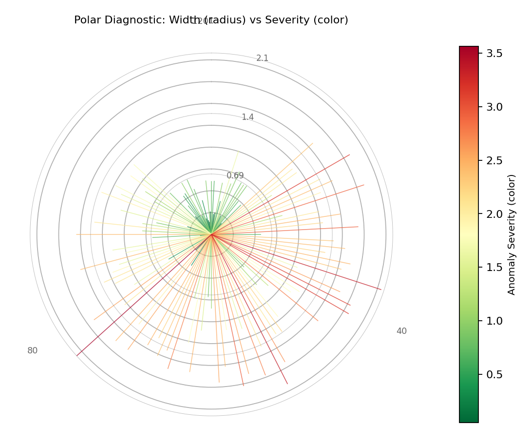
Long AND bright (red) spikes mark the most problematic sites: wide prediction intervals AND high severity. Long but green spikes indicate wide but well-placed intervals.

Analysis and Interpretation

This dual-encoding hedgehog reveals four quadrants of model behavior at once. Long + red spikes (south): the model produces wide intervals that still fail to contain the true value — the worst outcome. Short + green spikes (north): narrow intervals that remain well-covered — the ideal outcome. Long + green or short + red spikes indicate intermediate cases. The fact that most long spikes are also red (south) confirms that the calibration failure is strongly correlated with the model’s overconfidence in the high-severity zone.

---

Paired Spatial + Polar Diagnostic

The plot_paired_spatial_polar() function creates the two-panel composite that is the signature figure of the k-diagram spatial-polar framework. It directly reproduces the paired (a)+(b) and (c)+(d) panel layouts of the paper’s Figures 2 and 5:

• Left panel: Geographic scatter map colored by the metric.

• Right panel: Polar hedgehog diagnostic with the same metric and colormap.

Both panels share the same colormap, making the correspondence between geographic location and polar angle immediately readable.

Plot Anatomy

• Left — geographic map: Color = metric value. Optional site labels (map_label_sites) and ordering arrows allow the reader to trace polar angle back to geography.

• Right — hedgehog: Angle = latitude rank; radius = metric. Site labels at the circle perimeter (label_n_sites) cross- reference the map labels.

• Shared colorbar: One colorbar on the map panel applies to both.

---

Use Case 1: Single-horizon H1 paired view (replicates paper Fig 2)

The canonical paired view for a single forecast horizon. Three sites are annotated on the map so the reader can locate them in the polar diagnostic by their polar angle.

axes = kd.plot_paired_spatial_polar(
    df, "lon", "lat", "width_h1",
    order_by="lat",
    cmap="YlOrRd",
    colorbar_label="Interval Width H1 (m)",
    map_label_sites={0: "S1", 59: "S2", 119: "S3"},
    title="Paired View: H1 Interval Width (map + polar diagnostic)",
    figsize=(13, 6),
)

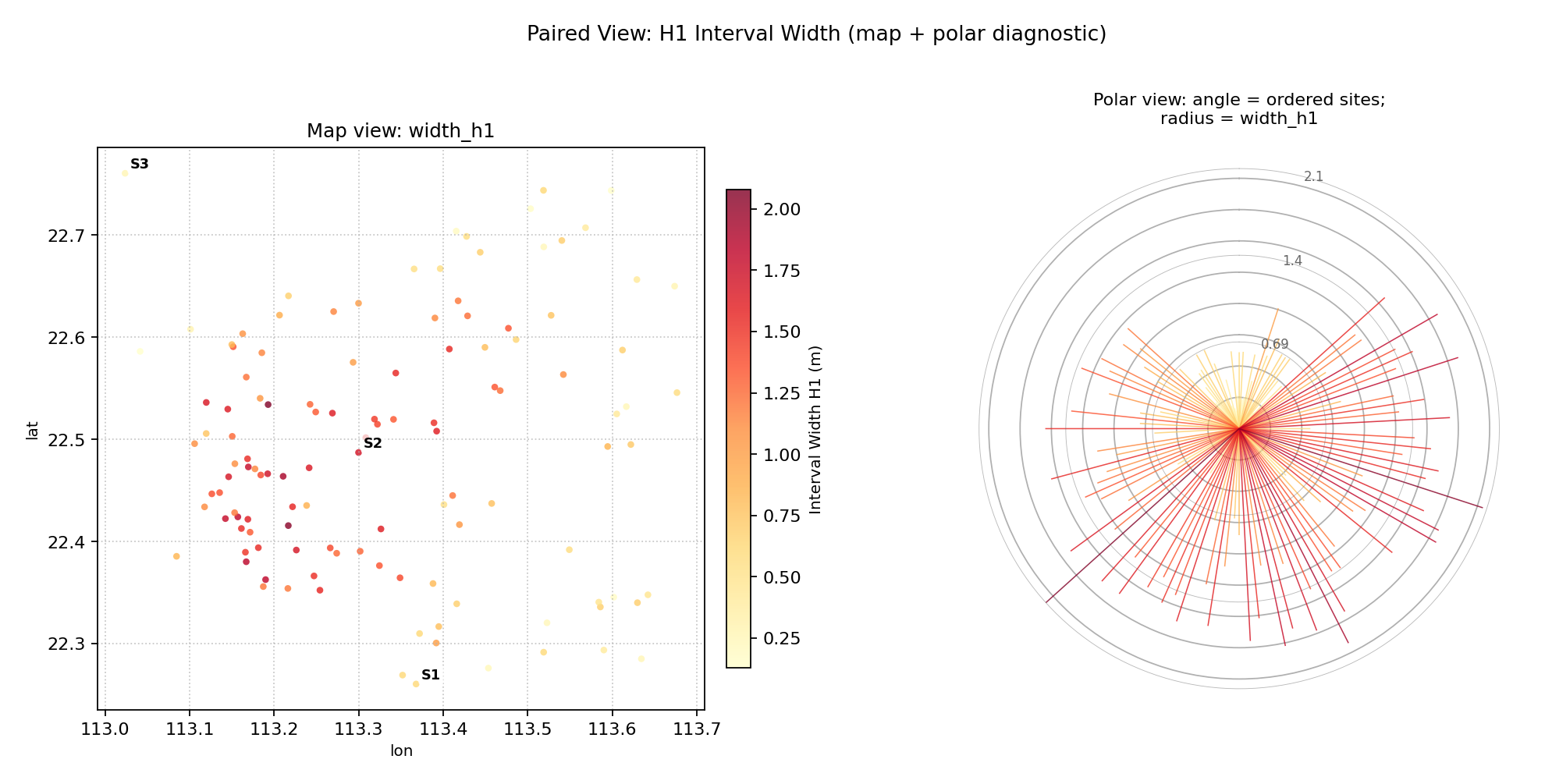
Left: scatter map of H1 width. Right: polar hedgehog. Site S1 (southernmost, rank 0) maps to the top of the polar circle; S3 (northernmost, rank 119) maps to just before the top after a full revolution. Long red spikes in the south confirm the hotspot.

Analysis and Interpretation

Reading both panels together:

1. Find a cluster in the map (e.g., the red-orange stations in the south-west near 113.20, 22.42).

2. Identify their latitude ranks — roughly ranks 0–30, placing them at polar angles 0°–90° (top-right arc of the circle).

3. Locate those angles in the hedgehog — the 0°–90° arc shows the longest, brightest spikes, confirming the map cluster.

This two-step reading is more powerful than either panel alone: the map shows where, the hedgehog shows how severe and what fraction of all sites share that profile.

---

Use Case 2: Multi-horizon paired view (replicates paper Fig 5)

Activating horizon_cols in the paired view places concentric rings in the polar panel while keeping the geographic scatter as the companion reference.

axes = kd.plot_paired_spatial_polar(
    df, "lon", "lat", "width_h1",
    horizon_cols=["width_h3", "width_h5", "width_h7"],
    horizon_labels=["H1", "H3", "H5", "H7"],
    horizon_colors=["#4393c3", "#f4a582", "#d6604d", "#a50026"],
    order_by="lat",
    cmap="viridis",
    title="Multi-Horizon Paired View (H1 inner ring to H7 outer ring)",
    figsize=(13, 6),
)

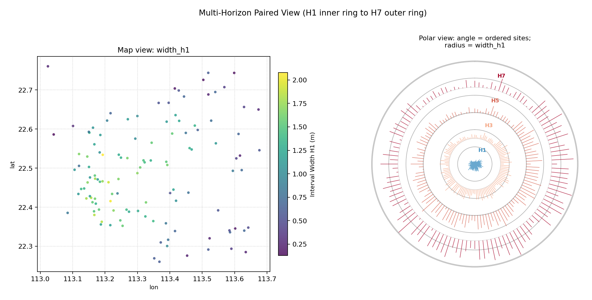
The polar panel shows four concentric rings (H1 blue inner to H7 red outer). Southern sites show dramatic outward ring growth; northern sites have thin, uniform rings. The map confirms which geographic cluster is responsible.

Analysis and Interpretation

The multi-horizon paired view answers the question “does uncertainty grow uniformly across the domain with forecast horizon?” in a single figure. The map (left) identifies the high-metric zone geographically; the ring diagram (right) shows that this zone also has the largest horizon sensitivity — the southern arc of the polar diagram is dominated by the wide red H7 ring, while the northern arc has thin, nearly equal rings across all horizons. This spatially non-uniform horizon growth is a key insight for model developers: improving long-horizon forecasts in the south requires a fundamentally different approach than improving short-horizon forecasts in the north.

---

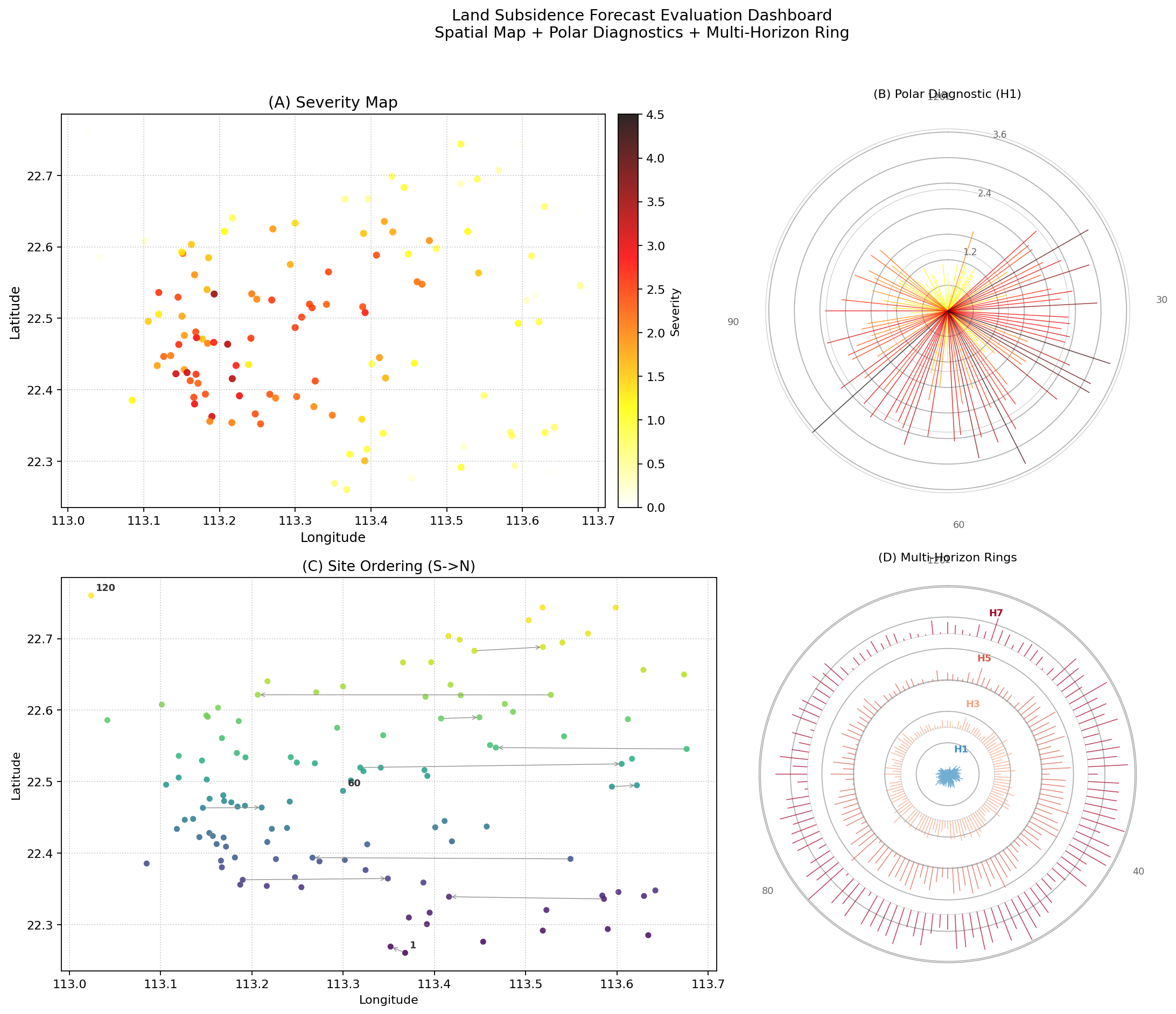
Application: Complete Spatial Forecast Evaluation Dashboard

In production, all eight spatial-polar functions combine into a single evaluation dashboard that guides the full diagnostic workflow:

1. Orient — the ordering map tells you how geography maps to polar angle.

2. Locate — the scatter / heatmap identifies where the metric is high.

3. Quantify — the polar hedgehog summarises the distribution of every site simultaneously.

4. Diagnose — the paired view reads map and hedgehog in tandem.

5. Compare — the comparison panel evaluates multiple models or horizons.

The following code assembles a compact 4-panel dashboard combining four of these views for the land-subsidence network.

import kdiagram as kd
import matplotlib.pyplot as plt
import numpy as np
import pandas as pd

# ... (build df with lon, lat, severity, width_h1-h7 columns)

fig = plt.figure(figsize=(15, 12))
fig.suptitle(
    "Land Subsidence Forecast Evaluation Dashboard\n"
    "Spatial Map + Polar Diagnostics + Multi-Horizon Ring",
    fontsize=13,
)

ax_map  = fig.add_subplot(2, 2, 1)
ax_pol  = fig.add_subplot(2, 2, 2, projection="polar")
ax_ord  = fig.add_subplot(2, 2, 3)
ax_pol2 = fig.add_subplot(2, 2, 4, projection="polar")

# (A) Severity scatter map
kd.plot_spatial_scatter(
    df, "lon", "lat", "severity",
    cmap="hot_r", vmin=0, vmax=4.5, s=35, alpha=0.85,
    colorbar_label="Severity", ax=ax_map,
    title="(A) Severity Map",
    xlabel="Longitude", ylabel="Latitude",
)

# (B) Single-horizon polar hedgehog
kd.plot_polar_from_spatial(
    df, "lon", "lat", "severity",
    order_by="lat", cmap="hot_r",
    colorbar=False, label_n_sites=5,
    title="(B) Polar Diagnostic (H1)",
    ax=ax_pol,
)

# (C) Site ordering reference map
kd.plot_spatial_ordering(
    df, "lon", "lat", order_by="lat",
    show_arrows=True, arrow_step=10,
    label_sites=[0, 59, 119],
    colorbar=False,
    title="(C) Site Ordering (S to N)",
    xlabel="Longitude", ylabel="Latitude",
    ax=ax_ord,
)

# (D) Multi-horizon ring diagram
kd.plot_polar_from_spatial(
    df, "lon", "lat", "width_h1",
    horizon_cols=["width_h3", "width_h5", "width_h7"],
    horizon_labels=["H1", "H3", "H5", "H7"],
    horizon_colors=["#4393c3", "#f4a582", "#d6604d", "#a50026"],
    order_by="lat", n_ring_labels=0, label_n_sites=4,
    title="(D) Multi-Horizon Rings",
    ax=ax_pol2,
)

fig.tight_layout()
fig.savefig("dashboard.png", dpi=150, bbox_inches="tight")

Analysis and Interpretation

Reading the four panels clockwise:

1. (A) Severity map identifies the spatial location of the failure hotspot: two bright clusters in the southern urban zone.

2. (C) Ordering map maps the ordering traversal onto the geographic coordinates: ranks 0–40 correspond to the southern cluster, so those sites will appear at polar angles 0°–120° in the hedgehog.

3. (B) Polar hedgehog confirms that the long, hot-colored spikes are indeed concentrated in the 0°–120° arc — consistent with the southern-cluster spatial assignment shown in (C).

4. (D) Multi-horizon rings reveals that this same arc also shows the fastest uncertainty growth with horizon — the H7 red ring dominates the south while remaining thin in the north.

Together the four panels deliver a complete, evidence-based narrative: the model’s failures are geographically concentrated in the southern urban zone, they are already the worst at H1, and they grow disproportionately fast with forecast horizon. A single aggregate coverage score would have hidden all of this structure.

Best Practice

Always present the ordering map (C) alongside the polar hedgehog (B/D). Without (C) the reader cannot know which angular arc corresponds to which geographic region. The paired view (plot_paired_spatial_polar()) automates this pairing, but the standalone ordering map is useful when the domain layout itself needs to be explained in detail.

---

For the mathematical background of the spatial-polar mapping, please refer to plot_polar_from_spatial — Core polar hedgehog diagnostic. For the API reference of all functions, see API Reference.